I. Scenario Modeling: Why We Build Scenario Atlases, Not Covariance Matrices

You build the world first, place views on them second, and optimize third.

Three key points:

• The optimizer is not the beginning of the portfolio process.
Before we place views or compute weights, we need a model of what can happen.

• A covariance matrix is a useful diagnostic, but a poor foundation.
It summarizes volatility and linear correlation, but it cannot show drawdowns, sequencing risk, regime shifts, or stress paths.

• Before deciding on which “world” your portfolio will live in the future - by weightening the probability of future paths - it is necessary to build a sufficiently rich set of possible worlds. Entropy Pooling (Block 2) and Portfolio Construction (Block 3) come later

Before you think about performing portfolio construction or even place an investment view on a portfolio, you need a model of what can happen to the assets in the future you want to invest in today. Most processes skip this step. They go straight from historical data to a covariance matrix, from a covariance matrix to expected returns, and from expected returns to portfolio weights. The model of what can happen is implicit — buried inside the Gaussian assumption, invisible in the optimization.

This series makes it explicit.

The broader architecture that connects risk identification, scenario generation, view integration and portfolio construction is described in Why Portfolio Construction Is More Than Optimization which describes the process of building and evaluating portfolios in four subsequent blocks. The article at hand is the starting point and focuses on the first question that architecture has to answer: What are the potential futures your portfolio might have to live in?

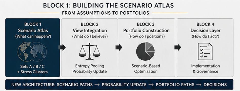
The central object of this series is not a covariance matrix. It is a scenario atlas: a structured collection of possible multi-year paths across assets, built from historical market data and extended with stress scenarios that history alone cannot provide. Views come later. Optimization comes later. First, we need to know what worlds we are asking our portfolio to survive.

This first article of my new flagship series explains why — and what we are building as necessary prerequisite for the subsequent steps of view implementation and portfolio constructoin.

A few honest words: While our approach will have a certain level of complexity, we still keep it rather simple in some aspects. Our framework is improvable in many areas, but for us it is intuition and the right mindset that is the heart of this series. The implementation can be found on Github. Find infos about the Technical & Data elements in the separate Technical Article of this series

The Problem with Covariance-First Thinking

First Of All: Using a covariance matrix is not wrong. It is a useful summary of how assets have moved together in the past - on average at least. It captures volatility. It captures linear correlation. It gives an optimizer something to work with.

The problem is not the covariance matrix itself. The problem is treating it as the foundation of the investment process — the primitive object from which everything else follows. When you start with covariance, you are already committed to a set of implicit choices that are rarely made explicit and are highly unrealistic:
You are assuming that second moments are the right summary of risk.
You are assuming that the correlations in your estimation window are a reasonable guide to future correlations.
You are assuming that a portfolio that looks efficient in covariance space will behave acceptably across the range of environments it will actually face.

None of these assumptions are obviously true. And more importantly, none of them are visible in the covariance matrix itself.

To be clear: even before we get to these deeper issues, the sample covariance matrix is a fragile object in its own right. With a limited number of observations and a meaningful number of assets, the raw estimate is noisy, ill-conditioned, and sensitive to outliers — problems that require shrinkage, robust estimation, or factor models to manage. We have written about this in detail here. But here is the more uncomfortable point: even a well-estimated covariance matrix faces a structural limitation that no amount of shrinkage can fix. It answers the wrong question.

Consider what a covariance matrix cannot tell you. It cannot tell you how deep a drawdown might be, or how long it might last. It cannot tell you whether the correlation between equities and government bonds will be negative or positive over the next three years — a question that turns almost entirely on the inflation regime. It cannot tell you what happens to credit spreads and equity volatility simultaneously in a liquidity crisis. It cannot represent the difference between a portfolio that loses thirty percent over six months and recovers, and one that loses thirty percent over six months and does not. These are not edge cases. They are the situations in which portfolio decisions actually matter.

The following table summarizes what a covariance matrix captures well and where a scenario atlas adds what it cannot provide.

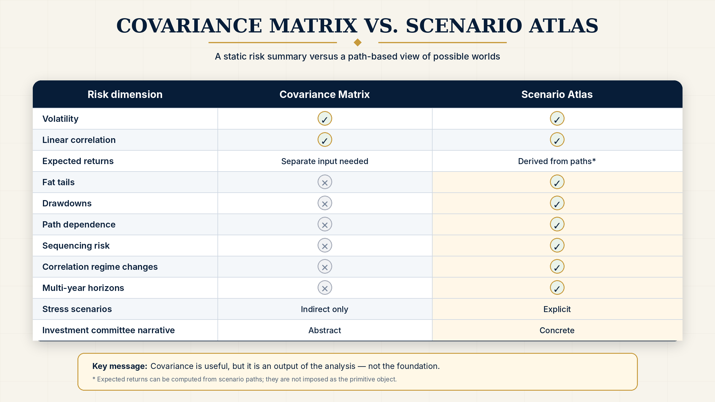
This series does not reject covariance. Volatilities and correlations are useful diagnostics, and we will compute them from scenario paths throughout. But they are outputs of the analysis, not its foundation. The foundation is a structured set of possible worlds.

What a Scenario Atlas Actually Is

A scenario atlas is a structured collection of possible futures — not point forecasts, not probability distributions in the parametric sense, but concrete multi-year paths across assets. Each path describes a potential future realisation or “world”: how equities moved, how bonds behaved, how credit spreads evolved, how the currency shifted — month by month, over a horizon of one, three, or five years.

The word atlas is deliberate. An atlas does not tell you where you will end up. It shows you the territory. It makes the range of possible destinations visible so that you can reason about them explicitly — which roads are likely, which are dangerous, which you have not prepared for.¹

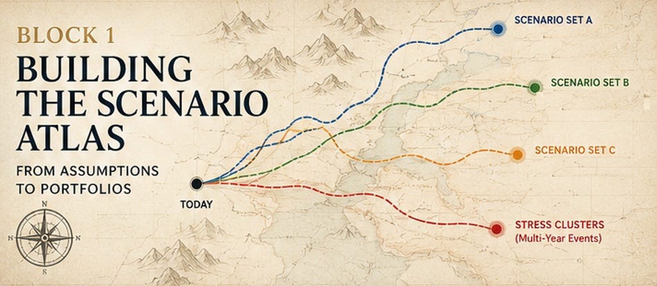
In this series, the atlas contains thousands of such paths, organized into three sets built with different methods. Each set reflects a different way of asking the same question: Given what history tells us about how markets move together, what worlds should our portfolio be prepared to face?

What makes this different from a covariance matrix is not a question of mathematical complexity. The distinction is one of transparency. A covariance matrix compresses the structure of market behavior into something algebraically convenient — a single object that an optimizer can work with directly. A scenario atlas keeps that structure visible. You can look at an individual path and ask whether it is plausible. You can count how many paths end in a drawdown of more than twenty percent. You can check whether your stress scenario of choice — stagflation, a liquidity crisis, a decade of financial repression — is actually represented, and with what weight.

This visibility is not just pedagogically convenient. It is what makes the framework governable. An investment committee can interrogate a collection of scenarios in a way that it cannot interrogate a covariance matrix. The question “which worlds are we not prepared for?” has a natural answer when the worlds are explicit. It has no answer when risk is summarized in a single matrix. ²

One more clarification before we go further. An atlas of possible worlds is not a set of forecasts. Building the atlas does not require a view on which world is more likely. That comes later, in Block 2 of this series, when we use Entropy Pooling to shift probability mass across the scenarios we have already built. The atlas and the views are kept separate — and that separation is the methodological core of this approach.

The Primitive Object: asset_paths

Every framework makes a choice about what to put at the center. In mean-variance optimization, the central object is the covariance matrix — everything else is derived from it or added to it. In this series, the central object is something different:

asset_paths # shape: S × H × N_assets

This is a three-dimensional array. S is the number of scenarios — in practice, several thousand. H is the horizon in months — we work with paths of up to sixty months. N_assets is the number of investable assets in the portfolio. This series models eleven investable assets and one auxiliary FX risk driver — EUR/USD — which is used to convert USD-denominated returns into EUR perspective.

In plain terms: asset_paths is a collection of possible futures, one slice per scenario, showing how each asset moved month by month over the full horizon.

The reason this is the right primitive object is a simple asymmetry. From paths, you can derive almost everything else you might want:

expected_returns = compute_means(asset_paths)
covariance = compute_covariance(asset_paths)
terminal_returns = compound(asset_paths)
max_drawdowns = compute_max_drawdown(asset_paths)
cvar = compute_cvar(asset_paths)

The reverse is not true. From a covariance matrix, you cannot recover paths. You cannot reconstruct drawdowns, sequencing risk, time-under-water, or the joint behavior of assets in a specific stress environment. The compression is irreversible.

This asymmetry is why we start with paths rather than moments. We are not giving up information to gain tractability. We are keeping the information and accepting a slightly different form of computation.

The paths in this atlas are built from historical market data — monthly returns from September 2010 to the present, giving approximately 189 observations. How exactly those paths are constructed from that data, and what assumptions each construction method makes, is the subject of the next four articles in this series.

Why Empirical-First

This series describes itself as empirical-first. That phrase needs unpacking, because it is easy to misread it as a rejection of models, or as a claim that historical data speaks for itself. Neither is true.

Empirical-first means that the starting point is the historical record of how assets have actually moved together — not a parametric model. We resample and reconstruct from observed market behavior rather than drawing from fitted distributions. History provides the raw material; the methods determine how we use it.

The alternative — parametric-first — would mean starting with a model. Assume returns follow a certain distribution. Estimate its parameters. Generate scenarios by drawing from that distribution. This is a legitimate approach, and in some settings the right one. But it carries a risk that is easy to underestimate: the model becomes a hidden assumption. The scenarios look like they came from data, but they actually came from a Gaussian copula, or a hidden Markov model, or whatever distributional choice was made. That choice shapes everything downstream, often invisibly.

Empirical-first makes the nature of the assumptions more inspectable. The building blocks are actual market observations — you can look at a resampled path and ask whether it is plausible, whether it corresponds to a real historical episode, whether the co-movements it contains make economic sense. That kind of inspection is harder to do with a scenario drawn from a fitted distribution, where the building blocks are model parameters rather than observable events.

But — and this is the point the phrase can obscure — empirical-first is not assumption-free. The assumptions do not disappear. They shift. And here the comparison with parametric approaches deserves more nuance than the empirical-first framing sometimes receives.

With a parametric model, the assumptions are written down explicitly. You specify a distribution, you write out the likelihood, you derive estimators with known statistical properties — consistency, asymptotic normality, confidence intervals. The model is on paper and, at least in principle, falsifiable. This is not a weakness. It is a genuine strength of the parametric approach. The formal explicitness of parametric assumptions is something empirical-first methods cannot fully match.

With empirical-first methods, the core assumption — that the historical sample is sufficiently representative of the range of plausible futures — is harder to make precise. It is less a formal assumption than a judgment call. You cannot write a likelihood for it. You cannot derive its sampling properties in the usual sense. In this specific way, the empirical-first framework is formally less explicit than its parametric counterpart, even as its building blocks are more directly inspectable.

The two dimensions are different and should not be conflated:

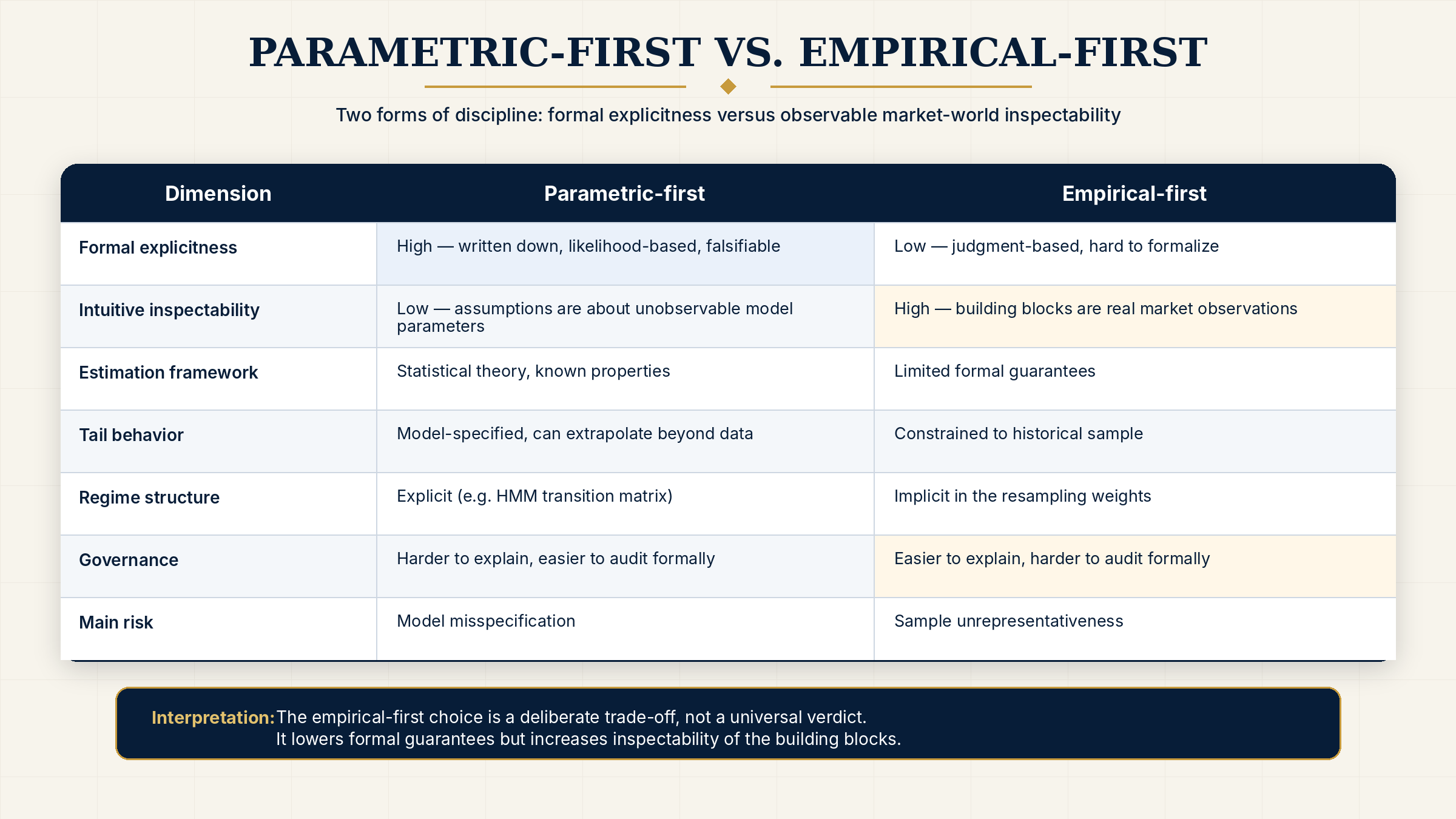
Neither column wins unconditionally. The empirical-first choice in this series is a deliberate preference, not a universal verdict. With approximately 180 months of data across eleven assets, we do not have enough observations to estimate a rich parametric model reliably — the curse of dimensionality bites hard in that regime. That tilts the balance toward empirical methods in this specific setting. In a different setting — more data, fewer assets, a well-understood return-generating process — the parametric approach might be the stronger choice.

We will also examine parametric alternatives directly. Hidden Markov models, copula-based generators, and factor-structured approaches each offer something the empirical sets do not — explicit regime structure, tail dependence modeling, cleaner separation of marginal and joint behavior. Understanding what they add, and what they cost, is part of taking the empirical-first choice seriously rather than treating it as the only reasonable one.

One more thing this series is not: anti-parametric. Parametric tools appear throughout — as volatility filters in Set C, as diagnostics throughout. The question is not whether to use models. It is where to put them. In this series, they are tools within an empirical framework, not the foundation of it. Whether parametric alternatives deserve a more thorough treatment of their own is a question we will return to separately.

What This Series Builds

Block 1 of this series produces a scenario atlas with three distinct sets of paths, each constructed using a different method. The sets are not competing alternatives — they are complements, each designed to answer a slightly different question about the range of plausible futures.

Set A — Synchronized Historical Block Bootstrap is the baseline. It resamples blocks of historical returns across all assets simultaneously, preserving the cross-asset structure that existed in each historical episode. No distributional assumptions, no latent states. Just history, resampled and stitched together into multi-year paths.

Set B — Conditional Similarity Resampling asks a refinement of the same question: are all historical periods equally relevant to where we are today? Set B weights historical episodes by their similarity to the current market environment — current yield levels, credit spreads, equity volatility, and other observable conditions. Periods that resemble today receive more weight. This is a state-dependent atlas without hidden Markov states.

Set C — Filtered Historical Simulation addresses volatility clustering. It separates the volatility state from the underlying market shocks, uses a filter to scale shocks to the current volatility environment, and then resamples the standardized shocks empirically. The shocks remain historical — no Gaussian draws — but their scaling reflects where we are in the volatility cycle.

In addition to these three sets, the atlas is augmented with a small collection of stress scenarios — structured multi-year paths representing environments that history alone underrepresents: deep stagflation, severe liquidity crises, prolonged financial repression. These are not point forecasts. They are modelling priors, assigned a small collective weight to ensure the atlas covers worlds it would otherwise miss.

All three sets share the same asset universe and the same horizon structure. Paths run to sixty months, and terminal returns are computed at twelve, thirty-six, and sixty months. This multi-horizon design allows the atlas to support both annual SAA reviews and longer-term strategic views.

The asset universe consists of eleven investable assets and one auxiliary FX risk driver:

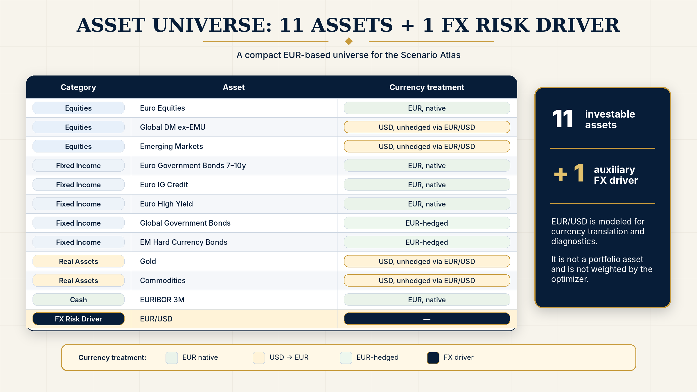
The data underlying the atlas runs from September 2010 to the present — approximately 180 monthly observations. The start date is determined by the earliest available proxy for Euro High Yield, the binding constraint in the asset universe. This shorter history than one might ideally want is part of the honest accounting this series tries to maintain throughout.

Limitations

This framework is deliberately transparent about its boundaries.

The historical return panel starts in September 2010. That gives a clean common sample across all assets, but it also means that some important worlds — including the 2008 financial crisis and earlier inflation regimes — are not directly present in the empirical sample. This is one reason the atlas later adds explicit stress clusters rather than pretending that history is complete.

The asset universe also uses practical public-market proxies, and the FX treatment is intentionally parsimonious: EUR/USD is the only explicit currency driver. These choices make the framework reproducible and explainable, but they remain approximations.

The detailed data sources, proxy choices, currency treatment, schema conventions and repricing logic are documented separately in Technical Note: Scenario Atlas Infrastructure.

What This Means for Your SAA

If you run a strategic asset allocation process, this series is relevant to you at three levels.

Diagnostic. Even if you never build a scenario atlas yourself, the framework changes what questions you can ask. Which historical environments does your current portfolio handle well, and which does it handle badly? What is the worst twelve-month path in a plausible set of futures? Which stress scenarios are absent from your current risk process? These questions have natural answers when possible worlds are explicit.

Governance. Investment committees are better at reasoning about scenarios than about covariance matrices. A portfolio that survives stagflation but struggles in a liquidity crisis is a comprehensible statement. A portfolio with a tracking error of 4.2% is not. The scenario atlas produces outputs that translate directly into committee language — not because they are simplified, but because they are structured around the questions committees actually care about.

Interested in ways to improve you decisions of your Investment Committee? Then check out our other series: The Allocator's Toolkit and The Irrational Committee.

Methodological. If you currently build your SAA around a mean-variance optimizer fed by a covariance matrix and a set of capital market assumptions, this series offers an alternative architecture. The optimizer still appears in Block 3, and the capital market assumptions still matter in Block 2. But the order of operations is different. You build the worlds first, place views on them second, and optimize third.

Key Takeaways

A covariance matrix is a useful diagnostic tool, but a poor foundation for strategic asset allocation. It compresses out exactly the information — drawdowns, path dependence, regime changes, stress behavior — that matters most in real portfolio decisions.

The primitive object of this series is asset_paths: a collection of possible multi-year futures across eleven assets, built from historical market data and structured into three complementary scenario sets.

Empirical-first does not mean assumption-free. The core assumption — that history is representative enough to resample from — is less formally explicit than a parametric model’s likelihood, but its building blocks are more directly inspectable. Both approaches involve genuine trade-offs.

The three scenario sets in Block 1 address different aspects of that trade-off: Set A is the synchronous historical baseline, Set B conditions on current market state, Set C accounts for volatility clustering. A small stress layer covers worlds history alone underrepresents.

Views come in Block 2. The atlas contains no investment opinion. Its purpose is to make the space of possible worlds visible before any probability tilts are applied.

Next: From Returns to Scenario Building Blocks

The next article in this series asks a more practical question: what exactly does history give us to work with, and what are its limitations as raw material for a scenario atlas?

Before we can resample historical returns responsibly, we need to understand their properties. Monthly returns are not independent draws from a fixed distribution. They exhibit autocorrelation, volatility clustering, fat tails, and time-varying correlations. These properties do not disqualify them as building blocks — but they determine how those building blocks should be used.

Disclaimer

This article is published for informational and educational purposes only. Nothing in this series constitutes investment advice, a recommendation to buy or sell any security, or an invitation to engage in any investment activity. The views expressed are those of the authors in their personal capacity and do not represent the views of any employer, institution, or affiliated organization.

All scenario construction, data handling, and methodological choices described in this series are illustrative. Past market behavior, however carefully analyzed, is not a reliable guide to future outcomes. Code published on GitHub is provided as-is, without warranty of any kind.

1. You should never forget: The world we are living in right now is the one which has “materialised” which was only one in a set of unlimited possible worlds that could have materialised. What about the other “world” that have not manifested?

Maybe a decision had only a few world where it would be successful. Would that be a wise decision only because it was successful in the world that manifested?

That’s a little deep for a quant finance article - i guess.

2. This will be a topic of one of the next articles in my series: “The Allocator’s Toolkit”