
Why Most Covariance Estimations Fail ... and How to Build One that Doesn't (Part 1)
This article introduces key concepts essential for accurately estimating covariance and highlights advanced techniques that enhance estimation accuracy, enabling you to achieve superior results.


Introduction
The best ideas about markets and timing are worth little, when there is no objective, unbiased routine to implement them into a portfolio. The crucial element to survive as an investor is to measure your risk correctly - in this regard, the covariance is still the main ingredient when portfolio risk is quantified. Therefore, after reading this article you will understand the essential concepts of the covariance and you will know superior approaches to estimate the covariance matrix more accurately in order to obtain better results in portfolio optimization and risk quantification. You will understand why it is so important to Clean Up your Covariance Matrix!
In this article, you will see how to capture the long-term characteristics of financial assets that are typically required for the construction of a strategic asset allocation (SAA). This assumes an investment horizon of at least 5 years. This focus allows the investor to look beyond specific parts of economic cycles and their conditional implications for return characteristics.
This article is Part 1 of our quest to show how to improve the estimation of the covariance matrix, which is still considered the most important parameter for portfolio construction in practice. Several advanced techniques will be presented which are easy to implement, commonly used in practice and highly superior to the simple sample-based estimation of the covariance matrix.
To improve understanding and you learning, we have provided the code for every graph and each technique on Github. Reading and using the code while following the article is highly advised.
The Relevance of the Covariance Matrix for Portfolio Optimization
Everyone who has touched the topic of portfolio optimization is familiar with the covariance matrix. In most cases, the covariance matrix is the key quantity to summarize the risk and (linear) dependencies of assets.1 You need an accurate and robust estimate because the optimized portfolio weights are based on it. If the covariance matrix is estimated poorly, you will over- or underestimate the risks of assets and their diversification effects. This should already be enough motivation to put some interest in its estimation.
However, the covariance matrix offers more than meets the eye. In fact, the biggest criticism of mean-variance optimization (MVO) is the sensitivity of portfolio weights to small changes in the input parameters (especially for varying expected returns). This aspect comes from the so-called “condition number” which is a statistical property of a (positive semi-definite) matrix and defined as follows:
The condition number is equivalent to the ratio of the largest and smallest eigenvalue of the covariance matrix.2 Using financial data, it is common to have some large eigenvalue on which the covariance matrix “loads” on. This is due to the stylized fact of high correlations between returns of similar assets. The “market factor” has often the dominant impact on returns and is mostly represented by the largest eigenvalue. However, you should put the focus on the smallest eigenvalues. The smallest eigenvalue will usually not represent much information, but often contains noise and estimation errors. Therefore, a high condition number will often be a sign that our estimation includes unnecessary elements which further reduces the already low signal-to-noise ratio in finance.
A high condition number leads to a very unstable inverse covariance matrix. This is a problem due to the fact that the optimal portfolio weights (in MVO) do not depend on the covariance itself, but on its inverse. Instability in this context means that small changes in the input parameters (e.g., expected returns) can have a large impact on the optimization output. This issue is not really a problem when using (non-parametric) Mean-CVaR optimization, which does not need a covariance inversion. That is another reason, why non-parametric Mean-CVaR is a more sound choice as an optimization algorithm than the classic mean-variance.
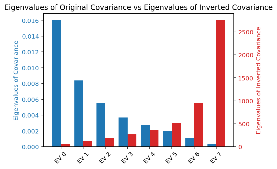
When the covariance matrix is inverted, its eigenvalues become the reciprocal of the original eigenvalues, while the eigenvectors remain unchanged. As a result, directions associated with small eigenvalues - potentially noise - in the original covariance matrix become dominant in the inverse. In the context of MVO, this means that these low-variance directions can disproportionately influence the portfolio weights. This sensitivity to small eigenvalues can lead to unstable solutions, which is the reason why regularization / shrinkage techniques are often used and much attention is warranted - especially if you believe that these eigenvalues are rather connected to noise than information. And portfolio weights driven by noisy elements does not sound right, does it? An example for 7 assets is given below. The smallest eigenvalue (EV 7) of the original covariance matrix has the largest eigenvalue in the inverted covariance matrix. Thus, it will have the largest impact on MVO.3
In short, a high condition number means that your covariance matrix is “on the knife edge” of numerical and statistical instability — any downstream computation that relies on it (not just portfolio weights) will be fragile and potentially misleading. This should be kept in mind not only for mean-variance optimization, but also for certain clustering algorithms, outlier detection, etc.
Financial Time Series Data: More Issues ahead
You have to be honest with youself about one aspect: Financial time series are difficult to handle. Before you can even think about estimation of the covariance, you have to make several assumption regarding the data generation process. At its core, you have to assume that the data is identically and independently distributed (IID)4 or at least ergodic5.
IID-ness is a very, very strong statistical assumption. Just to give you an indication which properties of financial time series can lead to a violation:
Serial correlation (autocorrelation) bias
Non‐stationarity / time‐varying moments
Volatility clustering & heteroskedasticity
Non-synchronous observation times
Structural breaks or regime shifts
This article does not focus on these elements, but the user should keep in mind that simply using covariance estimators on raw data might not be the best of idea. For example, using return data from equities or (open-ended) funds to estimate long-run parameters is often valid, as long as there is at least some hope that the returns are ergodic. For other financial instruments, like specific bonds or derivatives, you will need a fully fledged simulation framework - simply using past returns of bonds or derivatives does not work in practice.
Estimated vs. True Parameter
For the sake of simplicity, let’s assume that the data generating process is well-behaved (= at least ergodic). In most applications, the data generating process is not known. Therefore, the distribution and its moments must be estimated from the data. The most basic approach to use is the so-called “sample” covariance. In many cases, the usual decision is to estimate the covariance matrix with the sample covariance estimator like its some kind of commandment in statistics - despite its drawbacks.
The following is important and crucial to understand: There is a distinction between an estimator of a parameter and the true parameter itself. This is very relevant and easier to understand when considering the mean: The sample mean is an estimator of the true mean (unbiased, expected value) of a distribution. Another estimator is e.g. a trimmed mean, which is also an (robust but biased) estimator of the true mean of the distribution cleaned for outliers. This means that there are usually several estimators for a given parameter and those estimators can be tested under reasonable assumptions based on the concepts of estimation theory.
The Baseline: Sample Covariance
Following the argumentation from above, it is important to understand that the sample covariance is only one possible estimator of the true covariance. The estimator is common knowledge and reads as follows:
Using the sample covariance to estimate the true covariance is not the best idea. The following contains the key reasons which every quant should learn by heart. Although the arguments are presented as “distinct” elements, most of them are closely connected with each other.
Unbiased on average… but with high estimation error
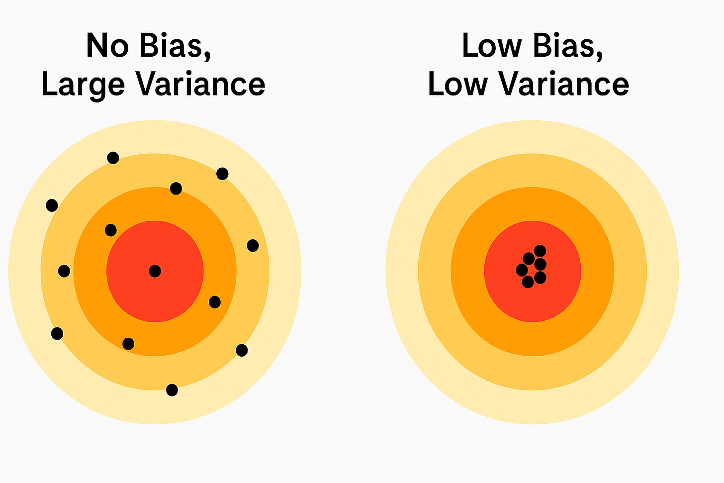
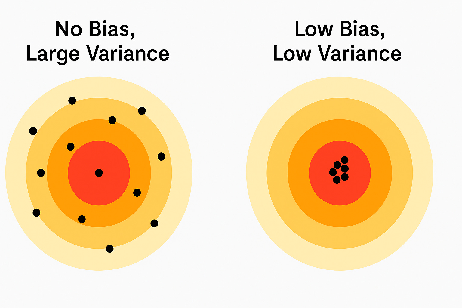
Sample covariance estimation is unbiased on average. But to obtain this property, it is paying a high price, as the estimation variance can be tremendous making it a highly unreliable estimate.
In practical settings, when data is limited, the sample covariance has the potential to be highly different from the true parameter.
Alternative approaches introduce a slight amount of bias, to reduce the variances significantly - which is often a better trade-off.
Equal-weighting of data points in estimation
Are all data points created equally?
Should you put more “weight” on some data points and less to others?In our opinion, there might be good reason to weight data point differently in the estimation process - due to some data points being too “extreme” or some just being too far away in the past.
Sample covariance (in its original form) implicitly assumes an equal-weighting by simply dividing the quadratic sum of deviations by the number of observations. This is not always appropriate.
High Variance in Small Sample, Curse of Dimensionality and Invertibility
When estimating a sample covariance, the number of parameter to be estimated from data quickly explodes:
\(\text{Number of free Parameter:} \\ \\ \underbrace{n}_{\text{variances}} \;+\; \underbrace{\binom{n}{2}}_{\text{covariances}} \;=\; n + \frac{n(n-1)}{2} \;=\; \frac{n(n+1)}{2}. \)As the number of parameter increases and the number of data points is fixed, the estimation becomes more noisy and less accurate.
If the number of variables (n) is larger than the number of observations (T), the sample covariance estimate becomes singular and the matrix cannot be inverted. This is an issue for any statistical analysis - but especially for many portfolio optimizers.
Ledoit-Wolf Effect
The Ledoit-Wolf effect highlights that the eigenvalues of the estimated sample covariance matrix tend to be more dispersed than the eigenvalues of the true data generating process.
For the sake of the argument, let us suppose the following example:
Given you have three financial instruments with identical volatilities and each being uncorrelated with the other.
What would you assume regarding the eigenvalue structure of the covariance matrix?
The eigenvalues should be identical in size…but due to issues introduced by the estimation approach, the eigenvalues are far from equal.
For a practical coding example see Github.
The estimation process leads to a too high dispersion among eigenvalues which increases the condition numbers. This in turn negatively affects the stability of many portfolio optimizers.
Sensitivity to Outliers
Sample covariance (and sample mean) are known to be highly sensitive to potential outliers.
Sample covariance is based on second‐moments and weights every point quadratically.
A single aberrant observation can dominate the estimation process, giving wildly inflated variances or spurious correlations.6
Therefore, the sample covariance is a non-robust estimator. It is therefore no surprise that the sample covariance is highly dependent on the specific samples used.
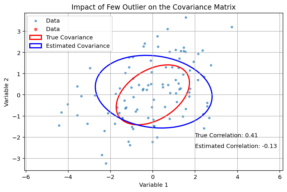
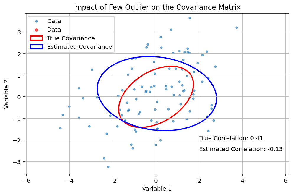
The following graph shows the impact of only 4 outliers in an dataset of 200 datapoints. In this example, a positive correlation in the data turns negative by the impact of only a few “bad datapoints”.
Let’s assume that those are two of your assets in an optimization: Using this (faulty) result, you will falsely assume high diversification effect between both assets which are not present in reality leading to a much higher portfolio risk than estimated.
Implicit assumption of normally distributed returns
Although, no specific assumption regarding the distribution are made, the sample covariance estimator has a clear connection to the normal distribution.
Let’s have a look at the maximum-likelihood estimator of Σ given a multivariate normal distribution is assumed. The estimator is:
\(\Sigma_{ML,Normal} = \frac{1}{T } \sum_{t=1}^{T} (r_{t} - \mu)(r_{t} - \mu)^\top \\\\ \)The equation of the estimator is almost identical to the sample covariance.
Decomposition: Covariances, Correlations and Volatilities
Before you will learn about the alternative estimators, it is important to stress the relationship of the covariance to the correlation and volatilities. As you (hopefully) know, combining correlations and volatilities generates the covariance matrix. The decomposition is as follows:
The covariance is therefore the combination of marginal and joint information. The important element to consider is that techniques to estimate the covariance matrix can - if necessary - also be separated into two steps:
1) Estimation of the correlation matrix and
2) Estimation of the marginal information (aka volatilities).
This decomposition is important in practice because in many cases, the difficulties with the covariance matrix arise mainly from the joint behaviour between random variables. Univariate volatilities are easier to estimate than the covariance between two random variables. This is because the covariance is the product of two univariate volatilities and the correlation coefficient which contains therefore more parameters (and uncertainty) that needs to be estimated from noisy data.
The decomposition provides the user with even more flexibility to apply alternative approaches to estimate the covariance “in one go” or - which is preferable in many cases - to focus on the estimation of the correlation matrix. This is also what we will be shown in the examples. As most estimators behave better when data is standardized, this will turn the covariance estimator into a correlation estimator. Afterwards, you can still combine the correlation with the volatilities to obtain the covariance matrix.
The Alternatives
At this point of the article, it is time to introduce alternative and superior techniques to estimate the covariance matrix:
Exponentially-weighted Sample Covariance
Outlier-Robust Sample Covariance
Graphical Lasso
Covariance shrinkage: Ledoit Wolf
Spectral Denoising
Factor models
To make a distinction between the approaches:
(1- 2) are approaches to (actually) estimate the covariance matrix, and the approaches (3 -6) are used to improve an already existing covariance matrix using shrinkage.
As an important remark: The most adequate choice will depend on your data set. Therefore, the “optimal” approach may differ.
Exponentially-Weighted Sample Covariance
The easiest approach is to drop the assumption that each datapoint should have the same “weight” in the estimation of the mean and the covariance matrix. The generalized equation to account for different weighting schemes is as follows:
\(\begin{align*} & \text{Sample Covariance with Flexible Probabilities } \\ & \mu = \sum_{t=1}^{T} p_t r_{t} \\ & \Sigma_{Sample} = \sum_{t=1}^{T} p_t (r_{t} - \mu)(r_{t} - \mu)^\top \\\\ & \text{where} \\ & \quad \quad r_t \in \mathbb{R}^n \quad \text{: Return vector at time } t \\ & \quad \quad \mu \in \mathbb{R}^n \quad \text{: Mean vector} \\ & \quad \quad \Sigma_{Sample} \in \mathbb{R}^{n \times n} \quad \text{: Covariance matrix} \\ & \quad \quad T \in \mathbb{N} \quad \text{: data sample (window) length} \\ & \quad \quad \sum_{t=1}^T p_t = 1\quad \text{: Flexible weighting probabilities (sum to one)} \end{align*}\)How to set the probabilities?
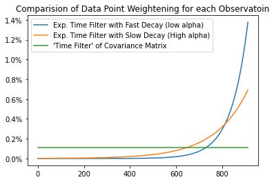
Many possibilities are available but overall two approaches dominate: (1) by some function of one or more state variable (= values of exogenous variables) or (2) by some function of time.7The examples in this articles show you how to perform time-dependent filtering and implicitly assume that more recent data points should have a higher weight. The time-filter is obtained by the following equation::
\(\begin{align*} & p_{t}|\alpha_{\mathit{HL}}\equiv pe^{-\frac{\ln(2)}{\alpha_{\mathit{HL}}}|t^{\ast}-t|}\text{,} \\ \\ &a: \text{half-life parameter} \end{align*} \)The decay depends on the half-life parameter alpha. The smaller the alpha, the faster the decay in probabilities is and, therefore the lower the weight of the more distant data points. This is shown in the graph below. The half-life parameter should not be set to high, to avoid using only the most recent data.
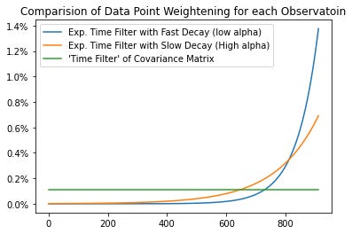
Overall, using this “flexible probability approach” to estimate the covariance matrix will not be enough to reduce the number of conditions. In fact, the condition might increase - therefore this approach should be combined with one of the shrinkage approaches presented below.
Outlier-Robust Sample Covariance
When estimating the mean, a common approach is to drop extreme outliers. While it is straightforward, to find outlier in a univariate setting (z-score), it can be more problematic in a multivariate one. But fear not, because the z-score is also defined in the multivariate case:
\(\begin{align*} &\text{Univariate Z-Score:} \\ &|z_{\textbf{x}}(x)|=\frac{x-\mu(x)}{\sigma(X)} \\ \\ &\text{Multivariate Z-Score (Mahalanobis Distance):} \\ &||z_{\textbf{x}}(x)||=\sqrt{(x-\mu(x))\Sigma(X)^{-1}(x-\mu(x))^{\prime}} \\ \end{align*}\)The approach is easy to implement:
(1) You define a threshold as number of points to be dropped (or sum of probabilities, when a flexible probability approach is used).8
Then, iterate over the following steps, until enough data points are dropped:(2.1) Calculate multivariate z-score for each data point
(2.2) Drop the datapoint with the highest z-score
(2.3) Recalculate the covariance matrix and means
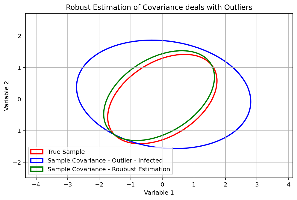
This simple approach is the equivalent to the “trimmed” mean in the univariate setting. The approach can be summarizes as follows:\(\begin{align*} &\textbf{Multivariate Outlier Trimming (Summary)} \\ &\text{Given: } X = \{x_1, x_2, \dots, x_n\} \subset \mathbb{R}^d, \quad \text{Threshold: } k \\ &\text{Step 1: Initialize } \mu = \frac{1}{n} \sum_{i=1}^n x_i, \quad \Sigma = \text{Cov}(X) \\ &\text{Step 2: Repeat until } k \text{ points removed:} \\ &\quad \quad \text{For each } x_i \in X, \text{ compute Mahalanobis distance: } z_i = \sqrt{(x_i - \mu)^\top \Sigma^{-1} (x_i - \mu)} \\ &\quad \quad \text{Remove } x_j \text{ such that } z_j = \max\{z_1, z_2, \dots, z_n\}\\ &\quad \quad \text{Recompute } \mu \text{ and } \Sigma \text{ on remaining points} \\ \\ &\text{Output: Trimmed dataset with updated } \mu \text{ and } \Sigma \end{align*}\)Obviously, using the Mahalanobis distance implicitly assumes that the data is normally distributed. While it is common to use the function EllipticEnvelope from the library scikit-learn , it can be easily implemented and adjusted based on the general idea presented above. This will be a topic in one of the next articles.
The graph below shows the impact of using robust covariance estimator, when outlier are presented. In the used (well-behaving) example, the robust estimator easily deals with the outliers. However, keep in mind, that this will not work as smoothly when real data is used.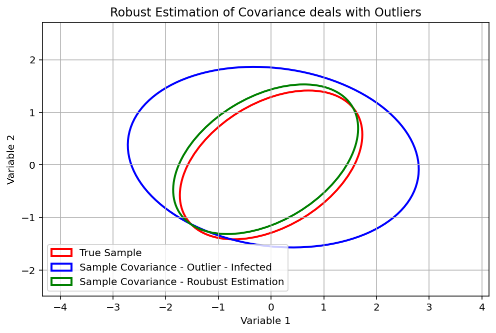
Failed to render LaTeX expression — no expression found
Graphical Lasso (GLasso)
The Graphical Lasso (GLasso) is a powerful technique used in statistical modeling to estimate the structure of a Gaussian graphical model—a network where nodes represent variables and edges reflect conditional dependencies. It’s particularly useful when dealing with high-dimensional data where traditional covariance estimates break down.
At its core, GLasso estimates a sparse inverse covariance matrix (also known as the precision matrix) by applying an L1 regularization penalty.9 The main idea is as follows: If the i, j -th element of an inverse covariance is zero, the variables i and j are conditional independent given the other variables. Shrinking the magnitude of coefficients in the inverse covariance matrix will therefore simplify the structure tremendously. Furthermore, the GLasso is one of the few approaches that directly tackle the inverse covariance matrix which is most relevant then Mean-Variance Optimization is used. In its practical application, Glasso provides a regularized inverse covariance matrix as shown below:
\(\begin{align*} {\Sigma^{-1}}_{\lambda}\equiv\operatorname*{argmin}_{{\Sigma^{-1}}}\,\operatorname{tr}({\Sigma^{-1}}\underline{{\Sigma^{-1}}})-\ln\det\nolimits({\Sigma^{-1}})+\lambda\Vert{\Sigma^{-1}}\Vert_{1}\text{.} \\ \text{where:} \\ {\Sigma^{-1}}: Inverse. Cov. Estimator \\ \underline{{\Sigma^{-1}}}: \text{Previous Estimate of Inv. Cov.}\\ {\Sigma^{-1}}_{\lambda}: \text{Glasso Estimate of Inv. Cov.} \end{align*} \)GLasso helps uncover hidden relationships while avoiding overfitting. If you’re working with datasets where variables outnumber observations—or just want a cleaner, more interpretable network structure—Graphical Lasso is a go-to method.
Covariance Shrinkage: Ledoit Wolf
Ledoit and Wolf (2004) suggest to shrink the covariance matrix to some target value in order to avoid perturbing the mean-variance optimizer. In mathematical terms, shrinkage reduces the ratio between the smallest and largest eigenvalue of the sample covariance matrix, so it increases the stability of the covariance matrix. To find the optimal shrinkage intensity, the authors provide the following solution:\(\begin{align*} &\Sigma^{*} = \rho^* \gamma \mathbf{I} + (1-\rho^*) \mathbf{\Sigma}\\ & \rho^* = \frac{ \hat{\beta}^2}{ \hat{\delta}^2} \\ & \text{with} \\ & \gamma := \frac{1}{n} \sum_{i=1}^T \Sigma_{ii} \\ & \hat{\delta^2} := || \Sigma - \gamma \mathbf{I} ||_F^2\\ & \hat{\beta}^2 := min( \bar{\beta}^2, \hat{\delta^2} ) \\ & \bar{\beta}^2 := \frac{1}{T} \sum_{t=1}^{T} || x_t^\top (x_t^\top)' - \Sigma ||_F^2 \\ & \text{where} \\ &x \quad \text{: Data of T x n dimension} \\ &\rho^* \quad \text{: Shrinkage intensity } \\ &\Sigma \quad \text{: Sample covariance matrix} \\ &\gamma \quad \text{: Multiplier for the identity matrix } \\ &\mathbf{I} \quad \text{: Identity matrix.} \end{align*}\)Although shrinkage provide a robust estimate of the covariance matrix which significantly improves the pure sample estimator, it is not free of doubts. As mentioned before, the aim of shrinkage is to handle the Ledoit Wolf effect which increases the condition numbers of a covariance matrix. Therefore, shrinkage makes many portfolio optimizer more robust. However, the key issue is the shrinkage intensity. When set too low, the shrinkage is ineffective to improve the condition number. When set too high, you risk to loose information in the covariance matrix with is needed to generate precise portfolio weights.
Spectral Denoising
Using the Ledoit Wolf shrinkage, you attempt to reduce the “noise” in the estimate generated by the estimation process. The problem with Ledoit Wolf is:
Can anyone be sure that you only eliminate noise? What is the right “degree” of shrinkage? Ideally, you want to get rid of the noise without eliminating information or signal in the data which is already low in financial data.
To give you some motivation: Laloux et al. reports that around 94% of the spectrum of an empirical correlation matrix estimated from the returns of the S&P 500 constituents is indistinguishable from the spectrum of a random correlation matrix. Therefore, denoising can make great sense - especially when the variables are similar (like are from the same asset class)!
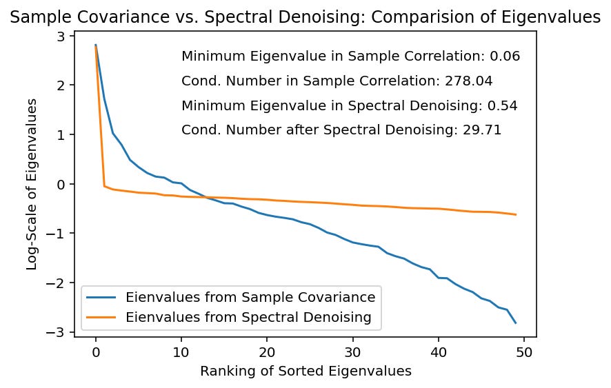
In this regard, spectral denoising can help. It uses Random Matrix Theory to eliminate noise, while keeping (most of) information in the data. What this approach does is to separate eigenvalues, which contain information from those eigenvalues which are more likely to contain noise. The separation is done by using the so-called Marchenko-Pasteur distribution (MPD). Eigenvalues, which contain noise follow the MPD and are mostly very small. Eigenvalues, which are significantly different from the distribution are assumed to contain information. The reader can compare spectral denoising with Ledoit-Wolf shrinkage by comparing a scalpel with an axe.\(\begin{align*} & \textbf{Marchenko-Pasteur Distribution of Eigenvalues:} \\ \\ & f[\lambda] =\begin{cases} & \displaystyle \frac{T}{N} \cdot \frac{\sqrt{(\lambda_+ - \lambda)(\lambda - \lambda_-)}}{2\pi \lambda \sigma^2}, & \text{if } \lambda \in [\lambda_-, \lambda_+] \\ \\ & 0, & \text{if } \lambda \notin [\lambda_-, \lambda_+] \end{cases} \\ \\ & \text{Maximum Expected Eigenvalue:} \lambda_+ = \sigma^2 ( 1+ \sqrt{N/T}) \\ & \text{Minimum Expected Eigenvalue:} \lambda_- = \sigma^2 ( 1- \sqrt{N/T}) \\ \\ & \text{Eigenvalues} \lambda \in [\lambda_-; \lambda_+] \text{ are consistent with random behavior} \\ \\ & \text{Eigenvalues} \lambda \notin [\lambda_-; \lambda_+] \text{are consistent with nonrandom behavior}. \end{align*}\)Therefore, you obtain a separation in the eigenvalues in two sets: The non-random eigenvalues do not follow the MPD - they are important for our analysis. What to do with the non-relevant eigenvalues? Your answer is called Constant Residual Eigenvalue Method. This means that the average across all eigenvalues with are associated with random behaviour is taken. Averaging across the lowest eigenvalues will lift up the lowest eigenvalue and thereby decreasing the conditions numbers:
\(\begin{align*} &\textbf{Constant Residual Eigenvalue Method:} \\ & \tilde{\lambda}_i = \begin{cases} \lambda_i, & \text{if } \lambda_i \notin [\lambda_-,\lambda_+] \\ \lambda_{\text{res}}, & \text{if } \lambda_i \in [\lambda_-, \lambda_+] \end{cases} \\ & \lambda_{\text{res}} = \frac{1}{k - 1} \sum_{i=1}^{k-1} \lambda_i \\ \end{align*}\)Some words of advice:
(1) It appears tempting to simply drop or eliminate the eigenvalues which looks random. However, this will reduce the rank of the covariance matrix and makes it (nearly) impossible to invert the covariance matrix.10
(2) This approach works best by using the correlation matrix - not the covariance matrix due to estimation issues of the MPD.
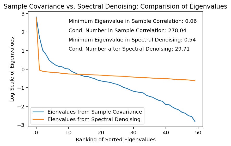
(3) Estimation of the MPD needs data points. In this framework, the data points are the eigenvalues. When the number of variables is low, the number of eigenvalues will be low, too. This can make it impossible to estimate the MPD n some settings. Therefore, you should use this process only when the number of variables is high (enough).Below, we illustrate one example demonstrating the impact of spectral denoising with the use of equity returns. You can see that the smallest eigenvalues are adjusted (increased), which severely reduces the condition numbers - and will ease some of the optimization / estimation difficulties.
Factor Models
In many settings, there are strong correlations in the data which are driven by variables in the background. Quite often, theory gives strong motivations that certain variables drive returns and stochastic processes. For example, nearly all stocks are commonly driven by one “market” factor.
The problem is that quite often you cannot be sure how to “quantify” those variables. Theory assumes they exist, but nobody really knows how to measure them correctly. In those cases “hidden” factor approach can be useful.\(\begin{align*} &\textbf{Factor Approach to Covariance Estimation:} \\ \\ & \Sigma_{factor} = \Delta\Delta^{\prime}+\Omega\text{,} \\ \\ \\ & \textbf{Optimization Problem:}\\ \\ &(\delta,\omega)\equiv\operatorname*{argmin}\limits_{\Delta,\Omega},\mathcal{D}(\mathit{\Sigma_{factor},\sigma}^{2})\text{.}\\ & \text{where:} \\ & \quad \quad \Omega \text{: Diagonal Matrix of } d\times 1 \text{ Vector} \\ & \quad \quad \Delta \text{: Full-Rank Matrix with Dimension } d \times k \\ & \quad \quad k \text{: Number of Hidden Variables} \\ & \quad \quad \mathcal{D} \text{: Distance Measure} \end{align*}\)As you can see, the factor approach decompose the covariance into two components: (1) common information across variables with can be represented by “hidden” factors, (2) idiosyncratic information which only corresponds to the specific variable. This decomposition crucially simplifies the structure (and the number of parameters), as you can focus on the small amount of hidden variables that “drives” the relationships.
Based on our experience, this approach highly decreases the condition numbers in many set ups. However, there are two important aspect to consider: How to set the number of hidden variables? How to estimate the factors? Estimation choice directly corresponds to choosing the distance measure. In many applications, the Frobenius Distance is used. In this case, optimization can be solved via principal axis factorization which is available in standard python packages.
The specification of the correct number of hidden variables is more difficult. To our knowledge, there are no clear cut approaches. We personally prefer to estimate several specifications by varying the number of hidden variables and then compare the covariance estimates based on the factor analysis and some another (robust) covariance estimate using the Frobenius norm (see in Github examples). Thereby you can detect when the covariance is highly different from the (robust) estimate. So you can increase the number of hidden variables, if the number is too low to adequately summarize relationships between variables.
Personally, we like to use this approach on the correlation matrix as we believe that focusing exclusively on the correlations appears to generate more robust results. This is the reason why the factor approach will be used in our examples.
Case Study:
Estimating the Covariance Matrix
As the remainder of this article, we will present a showcase of the presented estimators of the covariance matrix. The following setting is used:
Large number of Stocks (= Optimizing an Equity Portfolio)
50 Equities from the U.S. market between 2010 and 2024
Monthly data starting in 2010
Small number of Asset Class Indices (= Optimization a Multi-Asset Portfolio)
5 Asset Class Indices (3 equity indices, 2 bond indices) between 2010 and 2024
Monthly data starting in 2010
To obtain the data, Yahoo Finance is used. The code to download the data is integrated into the coding example on Github.
To evaluate the estimators, we apply the following strategy: The results are compared by looking at the obtained condition number. As highlighted before, a lower condition number is preferable especially for numerical stability. Afterwards, the differences between the estimated covariances are analyzed using the Frobenius norm. While you cannot - at least in this setting - tell which estimator is better or even “the best” in terms of quality and precision, you can at least say when two estimators are similar regarding the information content (e.g. when the Frobenius norm of the difference is low). Under similar estimators, you should prefer that one with the lower condition number.
Equity Example:
The graphs below show the results of using several methods to estimate the covariance matrix. The estimators are effective in reducing the condition numbers. The shrinkage approaches of Ledoit-Wolf, Glasso, Spectral Denoising and Factor Models are helpful in reducing the number of condition making matrix inversion and optimization more stable. Interestingly, although robust estimation can improve the quality of the coefficients / covariances, it fails at reducing the number of conditions. However, you can solve this issue by additionally apply shrinkage on the robust covariance estimator (see: Robust Estimation + Glasso).
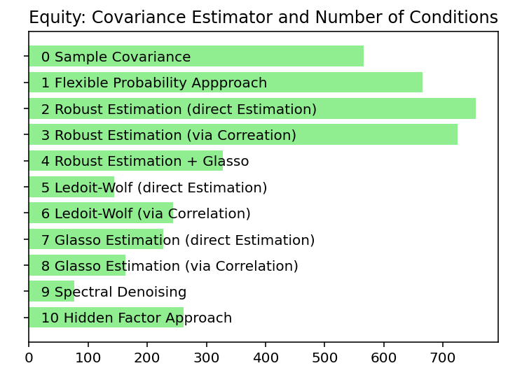
Its important to keep in mind that a low (or high) condition number does not say anything about the overall quality, such as a precise estimation of the true coefficients. In fact, you can reduce the condition number by simply setting the non-diagonal elements of the covariance matrix to zero - something that is not sound. However, given that “richness” of information in a covariance is contained while having a smaller number of conditions will lead to better results.
Therefore, having a look at the Frobenius (L2) norm of the differences between all pairs of covariance matrices is helpful. A smaller Frobenius norm (blue) means that two covariances estimates show little difference. You can see that the shrinkage approaches (columns 5-10) are rather similar to the sample covariance while having a far smaller condition number. These results are indicative that shrinkage on the data improves the numerical stability of the covariance estimates while preserving the majority of information.
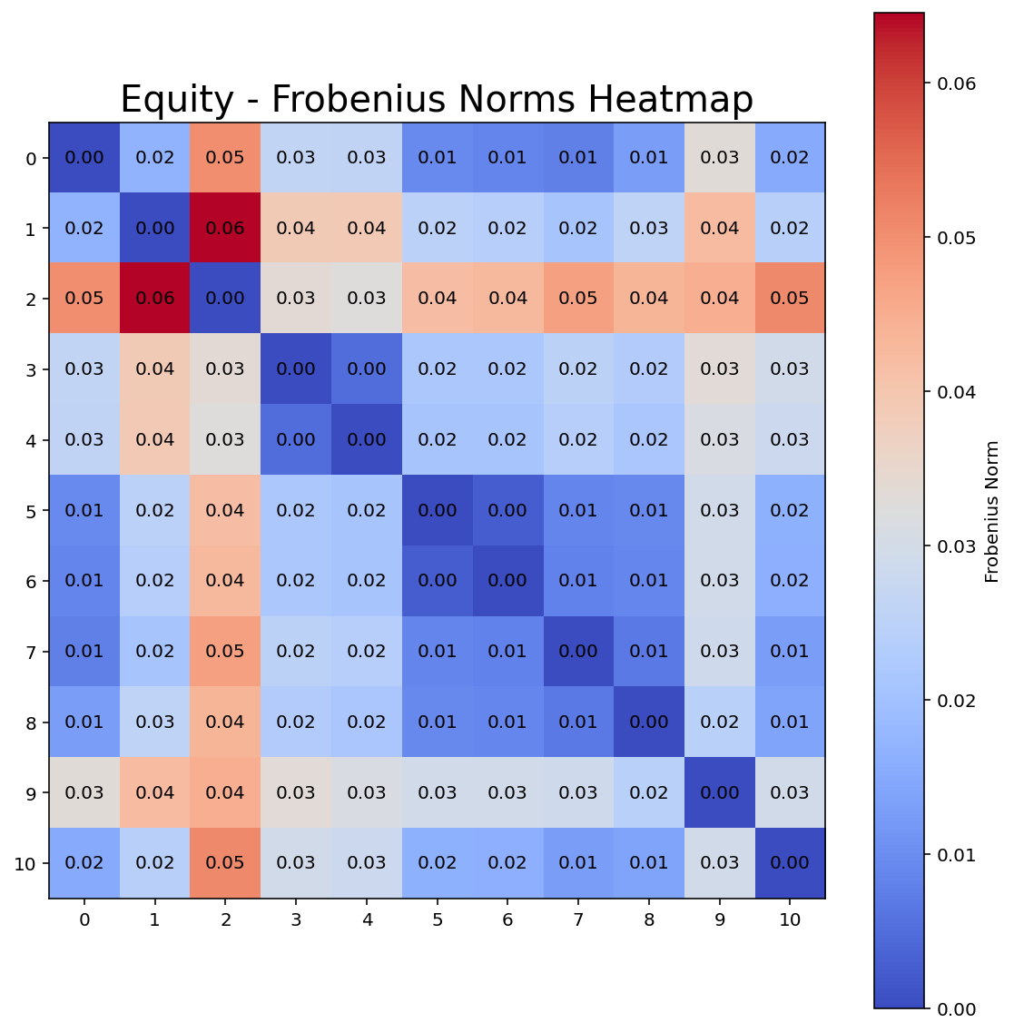
*The indices represent the estimators as presented in the graph of the number of conditions.
Multi-Asset Example:
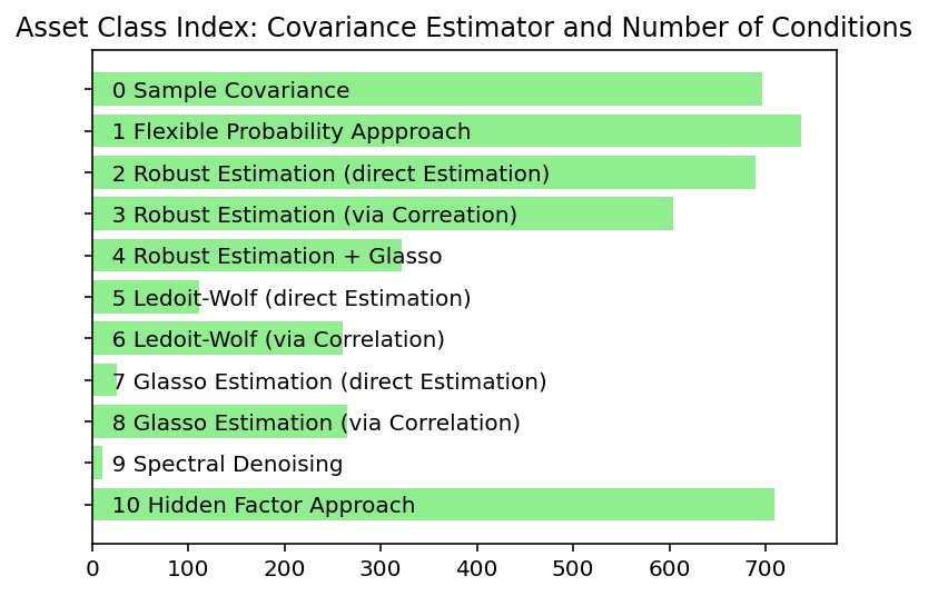
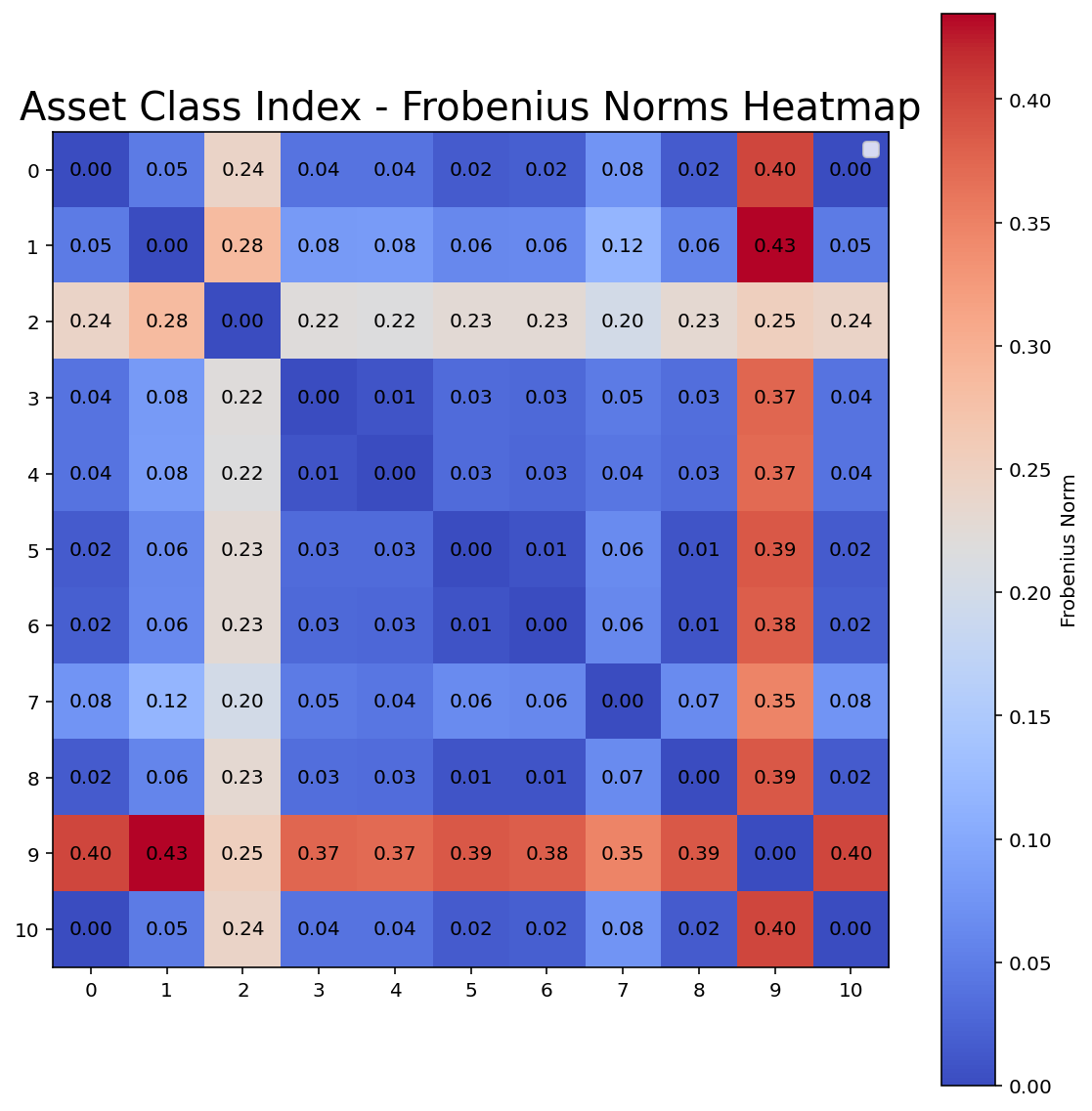
For strategical asset allocation, the second data set is more interesting, Once again, the pattern emerges that estimations without shrinkage generate high condition-number estimates. However, some of the shrinkage approaches are “overdoing” it, as the condition numbers are very small. This is a common situation, when the used shrinkage method may note be applicable with the settings / arguments used. A very low condition number (relative to the sample covariance) can reveal that the shrinkage is too strong which means that nearly all dependencies between variables are eliminated. This appears to be the case for Glasso, performed directly on the covariance matrix, and spectral denoising.
Therefore, this example gives insight that you can actually overdo shrinkage. The condition number and the covariance matrix itself should always be checked.
Summary
In this article, you have learnt that using the sample covariance can and will utterly fail - especially in portfolio optimization. It can lead to complete miscalculations of the dependencies and diversification effects between asset returns in some cases and can render portfolio optimization useless due to high sensitivity of the resulting portfolio weights. Please keep this in mind: You have been warned!
You have seen the key concepts of covariances. It is crucial to know that your data need to have certain characteristics. The methods used here can only applied when these characteristics (like ergodicity) are fulfilled. When this is not the case (as with derivatives and bonds) you will need more advanced techniques.
We illustrate several approaches to better estimate the covariance matrix. In practice, you have to consider two key aspects:
The best strategy to estimate the covariance matrix will depend on your data sample. There is no silver bullet that works every time - there is none in investing and none in covariance matrix estimation.
The various approaches can be combined to improve results. Why not try robust estimation and subsequently the factor approach? It might work and will tackle the issue from two different sides (outlier-reduction + structure simplification).
In Part 2 of this article, even more sophisticated approaches (e.g. marginal-copula estimation) will be presented. Additionally, you will actually see how to determine the quality of an covariance estimator in a coherent framework which you will be able to use in practice afterwards.
Before this article is concluded, we have one last question for the reader: How important is the choice of data frequency? Should monthly and daily data lead to identical correlations? Which frequency should you chose? Answering this question is far from trivial, but we will provide some guidance in Part 2.
Please keep in mind: Covariances only measure linear dependencies. For non-linearities, you can check out copula-based or entrophie-based distance metrics
https://en.wikipedia.org/wiki/Condition_number#Matrices
IID stands for Independent and Identically Distributed, and it's a foundational concept in probability, statistics, and machine learning:
1. Independence: Each data point (or random variable) does not depend on the others.
2. Identically Distributed Each data point comes from the same probability distribution.
→Makes estimation and inference easier and many algorithms (ML) depend on it.
A stochastic process is ergodic if statistical properties (like mean, variance, autocorrelation) computed from one long realization converge to the true (ensemble) expectations. It matters because it means that It matters in practice: If a process is ergodic, you don’t need multiple data sources — observing one over time is enough to understand the whole. This is allows use to estimate parameters from only one realized time series.
This means that the so-called “Influence Function” of the estimator is not “bounded”.
A single extreme data point can crucially change the entire matrix which is not a good feature of an estimator.
State and time-dependent probabilities can be combined using relative entropy techniques.
Apart from a fixed number of data points or a certain probability, you might also use the MV Z-Score as criteria. Because the MV Z-Score is chi-distributed, one might actually use a significance test to check for outliers. Obviously, this assumes that the data follow a multivariate normal distribution.
See https://www.stata.com/meeting/us21/slides/US21_Dallakyan.pdf
See Chapter 1 of De Prado’s “Machine Learning for Asset Managers” and the Summary of Random Matrix Theory for a discussion of spectral denoising.