Why Portfolio Construction Is More Than Optimization

From capital market assumptions to decision-ready portfolios.

Abstract

In this article, I argue that portfolio construction is more than just obtaining asset weights from an optimization. Robust portfolio construction is a broader decision architecture — from scenario generation and disciplined view integration to optimization and post-processing.

Three key points:

• Optimization is only one step.
A good portfolio process starts before the solver, with forward-looking scenarios, dependencies, regimes, and economic assumptions.

• Views should be integrated systematically.
Tactical views should not simply move weights around. They should transform the prior distribution into a posterior distribution in a disciplined and multivariate way.

• The output must be decision-ready.
A candidate portfolio needs to be tested for robustness, stress behavior, implementation, explainability, and mandate fit before it becomes a usable portfolio decision.

---

The most difficult part of portfolio construction is often not solving the optimization problem. It is defining the investment problem correctly in the first place.

In many investment discussions, portfolio construction is treated as if it were mainly a solver problem. Estimate expected returns, risks, and correlations. Define an objective function. Add constraints. Run the optimizer. Obtain portfolio weights.

This view is attractive because it is clean. It feels precise, quantitative, and disciplined.

But it is also too narrow.

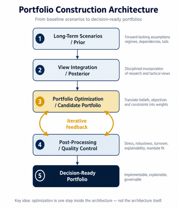
An optimizer can only solve the problem we have chosen to formulate. It does not decide whether the assumptions are economically sensible, whether the scenarios are rich enough, whether the views have been integrated consistently, whether the risk measure is appropriate, or whether the final portfolio can be implemented, explained, and governed in the real world.

A better way to think about portfolio construction is as an architecture that moves through four layers:

1. Generating long-term scenarios

2. Incorporating views

3. Optimizing portfolios

4. Post-processing the output into decision-ready portfolios

The first three steps are largely sequential. We start with a baseline view of the world, transform it with disciplined views, and then optimize based on the resulting distribution.

But the relationship between optimization and post-processing is different. It is iterative. The optimizer produces a candidate portfolio. Post-processing then tests whether this candidate is stable, explainable, implementable, and fit for the mandate. If it is not, the right response is not simply to manually polish the output. It may mean that the optimization problem itself needs to be reformulated.

In other words: A good optimizer produces weights. A good portfolio construction process produces decisions.

This article is not meant to be a technical deep dive into each component. It is a conceptual map of how these components fit together in a robust portfolio construction process.

This article is meant to serve as the conceptual roadmap for a future series on scenario generation, view integration, optimization, and post-processing.

---

1. Generating long-term scenarios: building the prior

Why forward-looking assumptions matter

It begins with the question:

What could happen - and with what probability?

Before we can optimize, we need a baseline distribution of possible future outcomes. This is the prior: a structured representation of what we believe the capital market environment could look like.

This prior should not be confused with a simple table of expected returns and volatilities. It is much more than that. It is a view on return distributions, risks, dependencies, tail events, and possible regimes.

The quality of this prior matters enormously. If the underlying scenario set is weak, no optimizer will rescue the result. The optimizer may still produce a mathematically precise answer, but it will be precise conditional on a poor description of the world.

This is particularly important for long-term capital market assumptions.

Historical averages can be a useful reference point, but they are a dangerous substitute for forward-looking assumptions. This is especially true for expected returns. Looking into the rear-view mirror can be misleading when valuations, interest rates, inflation regimes, profit margins, and structural growth drivers differ materially from the historical sample.

A simple example is equity returns. A historical average may include decades of valuation expansion. If one mechanically extrapolates that average, one may implicitly assume that the same valuation tailwind repeats itself. That is not a neutral assumption. It is a strong forward-looking claim disguised as historical objectivity.

Historical averages often mix realized cash flows, changing valuations, and regime-specific tailwinds. Treating them as neutral expected return estimates can therefore be misleading.

Good long-term capital market assumptions therefore need an economic foundation. They should ask which structural forces could shape future returns, risks, and dependencies.

Think about artificial intelligence. The relevant question is not simply whether AI is “positive for equities.” The more important question is how AI may affect productivity, margins, investment demand, energy consumption, inflation, and sectoral dispersion — and how these effects translate into asset-class and factor assumptions.

Demographics can influence labor supply, savings behavior, fiscal pressure, growth, real rates, and demand for safe assets. These are structural forces that may shape long-term distributions rather than short-term market views. Deglobalization and geopolitical fragmentation can affect supply chains, inflation, risk premia, regional growth, and correlation patterns in stress periods.

The main point is simple:

Long-term assumptions are not just forecasts. They are structured beliefs about the economic forces that may shape future return distributions.

---

Building a rich scenario universe

Once we accept that scenario generation is central to portfolio construction, the next question is how to build the scenario universe.

There are broadly two families of approaches: historical or resampling-based approaches, and parametric or simulation-based approaches.

Historical approaches preserve what has actually happened. They can capture real market movements, empirical co-movements, and observed stress periods. This is valuable. There is a certain discipline in forcing a model to confront real data rather than purely theoretical assumptions.

Resampling-based approaches can be useful in this context because they allow us to generate many possible paths while staying connected to empirical market behavior. A good example of this type of thinking can be found in Kristensen and Vorobets (2025) on scenario-based portfolio construction and resampling approaches.

But historical approaches also have a limitation: the past may not contain the full range of future states that matter. A historical sample may not include enough inflation shocks, geopolitical stress regimes, liquidity crises, or correlation breakdowns. It may also overweight regimes that are no longer representative.

Parametric and simulation-based approaches address a different problem. They allow us to design distributions more explicitly. We can model higher moments, fat tails, skewness, kurtosis, changing volatility, and different dependency structures. We can also introduce regime-based dynamics, for example through Markov-type regime
models.

This matters because portfolio construction is not only about average returns. It is also about what happens in unusual states of the world.

Consider a simple regime example. In a benign growth regime, equities and credit may perform well, volatility may be low, and correlations may look stable. In an inflation shock regime, rates, equities, commodities, and currencies may behave very differently. In a geopolitical stress regime, volatility may rise, correlations among risky assets may increase, and safe-haven assets may react differently than in normal times.

A richer scenario universe can include these different states. That is especially important if the next step is to incorporate views using methods such as Entropy Pooling.

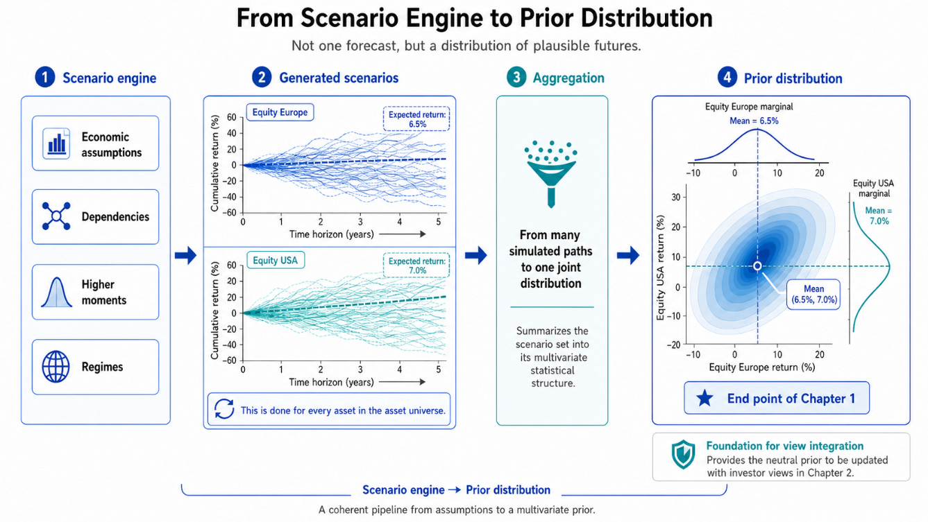
Regardless of historical or parametric scenario generation, the aim is not to predict one future. It is to build a rich, economically grounded representation of plausible future states.

A useful scenario universe should contain different states of the world - including different growth, inflation, risk and correlation regimes. This is essential because Entropy Pooling can only reweight the scenario universe that is already available.

---

Assets, factors, and dependencies

Another design choice is whether scenarios and views are expressed at the asset level, the factor level, or both.

Factors are often the natural language of views. A view on real rates, inflation, credit spreads, the US dollar, volatility, or equity risk premia is usually easier to express as a factor view than as a direct asset allocation decision. This can make the link between research and view integration cleaner.

Assets, however, are the language of implementation. Final portfolios are built from asset classes, funds, indices, or instruments. Asset-specific characteristics — especially in equities, where region, sector, valuation, currency, and index composition matter — cannot be ignored.

A robust architecture should therefore connect both levels: factors for economic interpretation and view formulation, assets for implementation and portfolio construction.

Scenario generation is not only about individual asset behavior. It is also about joint behavior.

Expected returns may get most of the attention, but dependencies are often just as important. Covariances, correlations, tail dependencies, and regime-dependent co-movements shape the actual diversification properties of a portfolio.

This is why covariance modeling is not a technical side issue. It is part of the scenario architecture.

Correlations are not stable. They can change across regimes. They often rise in stress periods exactly when diversification is needed most. Tail dependencies can matter more than average correlations. If the scenario model fails to represent these features, the optimizer will work with an incomplete picture of risk.

I have written a separate article about covariance modeling and why dependency estimates matter for portfolio construction.

For the purpose of this article, the key point is this:

A scenario model is not only a model of returns. It is also a model of dependencies.

---

2. Incorporating views: from prior to posterior

A prior scenario distribution is only the starting point. In this context, tactical views are not meant as ad-hoc tilts. They are disciplined modifications of the strategic prior.

Investment teams rarely want to optimize purely on an unconditional baseline distribution. They have views for the short- or medium-term. These views may come from CIO discussions, investment committees, tactical asset allocation decisions, macro analysis, and so on.

The question is not whether views should exist. They always do.

The real question is: how they enter the portfolio construction process.

This is where judgement and discipline meet. Views are often an expression of judgement. But without structure, judgement can easily become inconsistent, biased, or impossible to evaluate. A disciplined portfolio construction process should define how judgement enters the distribution.

Views are not a substitute for structure. They become useful only when they are embedded in a disciplined probabilistic framework, such as Entropy Pooling.

---

SAA as anchor, TAA through views

One way to think about the relationship between strategic and tactical asset allocation is the following:

The long-term scenario distribution represents the strategic baseline. It reflects structural capital market assumptions and long-term beliefs. Tactical views then transform this prior into a posterior distribution.

In this architecture, strategic asset allocation (SAA) provides the anchor while tactical asset allocation (TAA) enters through views. This matters because tactical allocation should not be a disconnected overlay that simply moves portfolio weights around. It should be a disciplined expression of views within the same broader portfolio construction architecture.

In that sense, the TAA portfolio is not merely “the portfolio after some tactical tilts.” It is the portfolio that reflects tactical views in a structured way.

---

Black-Litterman and Entropy Pooling

There are different ways to integrate tactical views.

Black-Litterman is especially useful for combining prior return estimates with absolute or relative return views. Entropy Pooling is more general in the context discussed here, because it works directly on the scenario distribution and can incorporate views beyond expected returns.

Entropy Pooling starts with a prior scenario distribution and changes scenario probabilities so that the posterior distribution satisfies the specified views while remaining as close as possible to the prior.

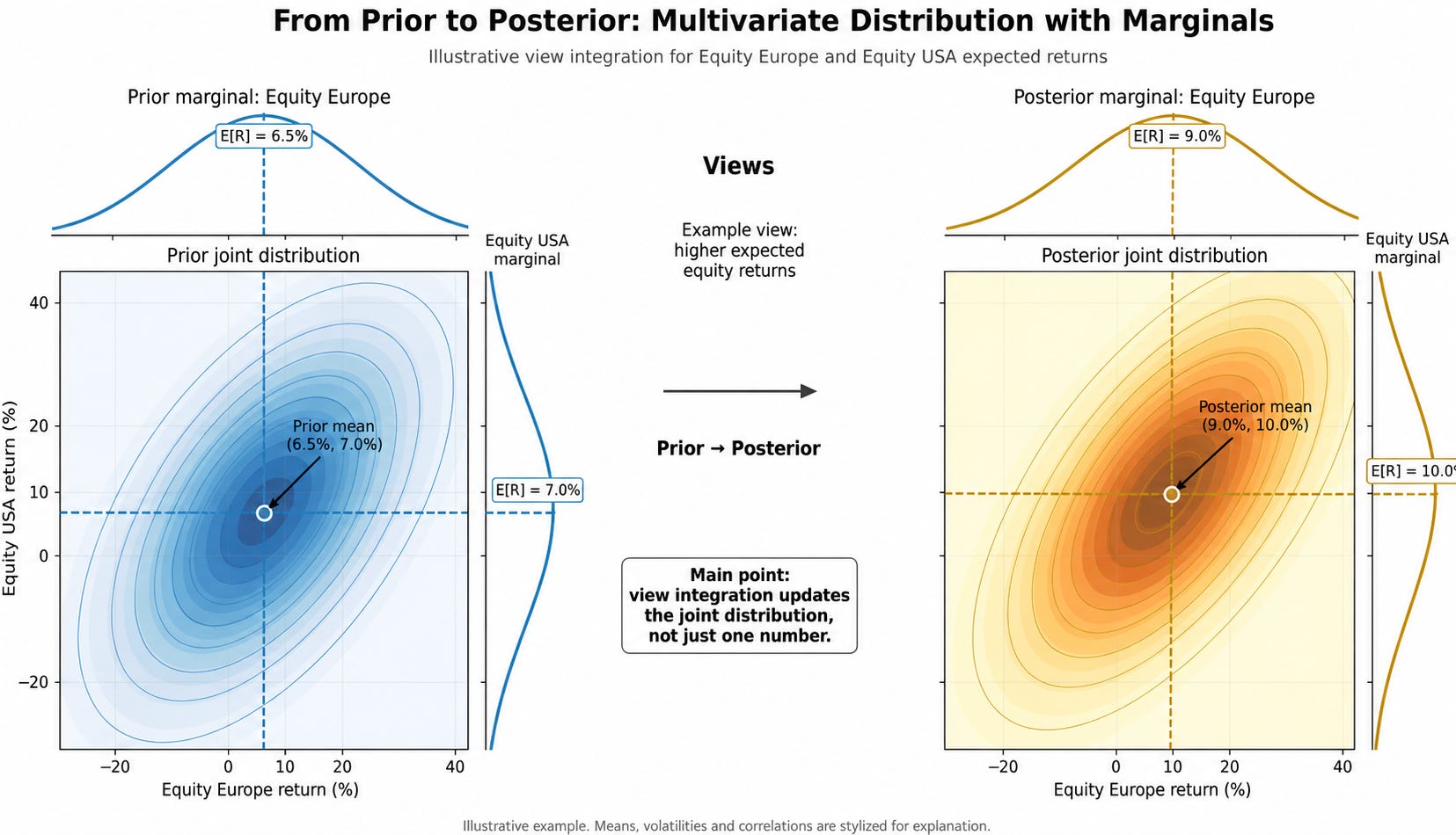
Views may concern:

• expected returns

• relative performance

• volatility

• correlations

• tail risks

• factor outcomes

The key advantage is that Entropy Pooling works directly on the scenario distribution. It can therefore incorporate a broader set of views than expected returns alone.

This does not mean that Entropy Pooling is always superior in every context. But for an architecture that starts with a rich scenario universe and wants to express views in a multivariate way, it is a very powerful tool.

---

The real value of view integration

The main value of view integration is not merely that expected returns can be changed.

The more important point is that these changes can be made consistently within the multivariate distribution.

A naive view might say: increase the expected return of one asset class. But in reality, an investment view often implies more than that. It may also imply changes in volatility, correlations, tail risks, or regime probabilities.

Consider a geopolitical stress scenario. A view on geopolitical escalation is not only a return view. It may imply higher volatility, changing correlations between equities, bonds, currencies, gold, and commodities, as well as higher tail risks.

In such a case, simply adjusting one expected return is not enough. The view should affect the joint distribution.

This is exactly where a scenario-based view-integration framework becomes valuable.

This is also why the prior scenario universe matters so much. If the prior does not contain enough sufficiently different scenarios, Entropy Pooling has little room to express such views. It can reweight what exists. It cannot fully compensate for a poorly designed scenario universe.

---

3. Portfolio optimization: from beliefs to candidate portfolios

Only after the prior has been built and views have been integrated does optimization enter.

At this point, we have a posterior distribution. This distribution reflects long-term assumptions and disciplined views. The optimizer can now translate this distribution into a candidate portfolio.

This step is important. Optimization is not the enemy. It is a powerful way to formalize trade-offs between return, risk, constraints, and objectives.

But optimization itself is already full of design choices.

What are we optimizing?

• mean-variance efficiency?

• expected return for a given level of downside risk?

• CVaR or other downside-risk measures?

• tracking error?

• turnover?

• robustness?

• multiple objectives in a sequence?

Which risks matter? Which constraints matter? Which trade-offs are acceptable? Which objective is appropriate for the mandate?

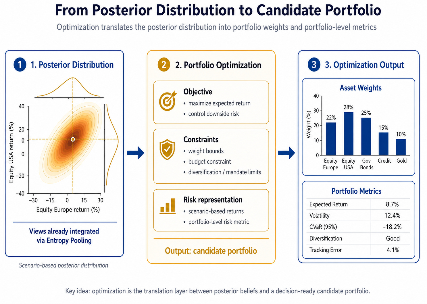
A portfolio for a long-term strategic allocation problem may require a different objective than a tactical implementation portfolio. A UHNWI portfolio with illiquid assets and client-specific constraints may require a different design than a model portfolio without legacy exposures.

In a previous article, I discussed lexicographic optimization as one way to deal with multiple objectives in portfolio construction. The broader point is that optimization itself is already embedded in a set of design choices: what we optimize, in which order, under which constraints, and for which purpose.

The optimizer transforms beliefs into candidate portfolios. But it does not automatically transform candidate portfolios into good decisions.

Optimization is only as useful as the design choices around it: the assumptions, objectives, constraints, risk measures, and quality controls that define the problem.

---

4. Post-processing: from candidate portfolio to decision-ready portfolio

The output of an optimizer is not the end of portfolio construction.

It is a candidate.

The next question is:

Can this portfolio actually be implemented, explained, monitored, governed, and defended?

This is what I mean by post-processing. Not cosmetic polishing. Not manual tinkering. Not making the output look nicer.

Post-processing is the quality-control layer that turns optimized portfolios into decision-ready portfolios.

In this sense, post-processing is not an override of the optimizer. It is a structured review of whether the optimized candidate portfolio is fit for decision-making.

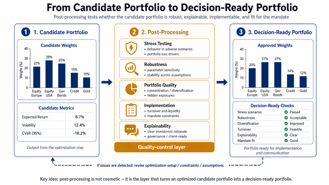
A decision-ready portfolio requires more than expected return and volatility.

It should be tested against stress scenarios. How does the portfolio behave under relevant adverse conditions? What drives the losses? Which assets or factors dominate the stress exposure?

It should be robust to uncertainty about the future. Does the portfolio only work in the baseline scenario? Or does it remain plausible across alternative regimes?

It should be robust to parameter uncertainty. What happens if expected returns change slightly? What if correlations move? What if volatility assumptions are wrong? If small input changes lead to large allocation changes, the portfolio may not be robust. It may be nervous.

It should be checked for concentration and hidden exposures. Does the optimizer create extreme weights? Are there unintended factor bets? Are diversification benefits real or only apparent?

It should be implementable. Turnover, liquidity, costs, operational constraints, and mandate restrictions matter. A mathematically attractive portfolio that cannot be implemented is not a successful outcome.

It should also be explainable.

This is particularly important in advisory, investment committee, and UHNWI contexts. A portfolio that cannot be explained is fragile, even if it looks attractive in a model. The decision-maker must be able to explain why the portfolio looks the way it does, which assumptions drive the result, what role tactical views play, and how the portfolio behaves under uncertainty.

Client-ready does not mean simplified. It means that the portfolio can be stress-tested, implemented, explained, monitored, and governed in the real world.

---

The iterative link between optimization and post-processing

The relationship between optimization and post-processing is not purely sequential.

It is iterative.

If post-processing shows that the candidate portfolio is stable, explainable, implementable, and aligned with the mandate, the process can move forward.

But if the portfolio is too concentrated, too sensitive, too difficult to explain, too costly to implement, or too weak under relevant stress scenarios, the solution is not simply to adjust the weights manually.

The right question is deeper:

• Was the objective function appropriate?

• Were the constraints correctly specified?

• Was the view too strong?

• Was the prior scenario universe rich enough?

• Were dependencies modeled properly?

• Was the risk measure aligned with the mandate?

• Did the optimization problem express the real investment problem?

This is why post-processing matters. It can reveal that the investment problem needs to be reformulated.

A serious post-processing layer does not simply polish the output. It challenges the formulation of the problem.

---

Conclusion: Portfolio construction is an architecture

Portfolio construction is therefore not the act of running an optimizer.

The optimizer is indispensable. But it is only one step in the architecture.

The process starts with a prior: a forward-looking scenario distribution grounded in economic assumptions. It then incorporates views to form a posterior distribution. Optimization translates this distribution into candidate portfolios. Post-processing tests whether these candidates can become decision-ready portfolios.

This is the difference between optimization and portfolio construction:

A good optimizer produces weights.

A good portfolio construction process turns scenarios, views, constraints, and uncertainty into portfolios that can be implemented, explained, monitored, and governed.

That is why portfolio construction is more than optimization.

---

Further reading / related notes

• My related notes:

  • A Better Portfolio Optimization Framework: Risk Constraints First, Lexicographic Selection Second

  • Why the Optimal Portfolio Is Often Not the Best

  • Why Most Covariance Estimations Fail ... and How to Build One that Doesn't (Part 1)

• Covariance modeling:

  • Ledoit & Wolf (2004): A well-conditioned estimator for large-dimensional covariance matrices

• Scenario generation and resampling:

  • Kristensen, L. & Vorobets, A. (2025) Time- and State-Dependent Resampling

  • Vorobets (2025): Time- and State-Dependent Resampling

• Regime switching:

  • Hamilton et al. (2005): Regime-Switching Models

• View integration

  • Meucci (2008): Fully Flexible Views: Theory and Practice

  • Idzorek (2004): A Step-by-Step Guide to the Black-Litterman Model

• Downside-risk optimization:

  • Rockafellar & Uryasev (2000): Optimization of Conditional Value-at-Risk

---

Disclaimer

This article is for educational purposes only and does not constitute investment advice or a recommendation. All examples and figures are illustrative and intended to explain the portfolio construction process conceptually. They do not represent investment recommendations. Views expressed are my own and not necessarily those of my employer.