The Frequency Trap: Why Daily Covariances Can Break Monthly Portfolios (Part 2)

Covariance Series — Horizon matching, scaling myths, and a practical recipe.

0) Abstract

If you rebalance monthly but estimate covariances from daily returns (and then multiply by 21), you often end up comparing apples to oranges. While you are actually interested in the risk forecasts of one month (or even more), the usage of daily data will not be aligned with our horizon. The result is: You get different portfolios and different risk forecasts, even when the estimator is identical. Even worse: You might obtain a portfolio for a “day trader”, while you are actually interested in a diversified low-frequency portfolio.

This post separates horizon (what you want to forecast) from frequency (how you measure returns), shows why “monthly = 21×daily” breaks under real market dynamics, and ends with a practical recipe you can ship into production. With this information, you will be able to decide on the compromise between using “more” data vs “better-aligned” data to your specific investment horizon.

Takeaways:
(1) Rebalancing horizon defines the covariance you need.
(2) Scaling is not a free pass.
(3) Fix the horizon first—then compare estimators (Part 3).

To improve understanding and you learning, we have provided the code for every graph and each technique on Github. Reading and using the code while following the article is highly advised.

1) Introduction: The Trap

In Part 1 we showed that the sample covariance matrix is unstable—and why shrinkage, denoising, and factor structure can help (while matrix norms and condition numbers are not portfolio-quality metrics by themselves).

Part 2 picks up the question that usually gets ignored in practice: how much does data frequency (daily vs. monthly) matter when the portfolio horizon is monthly?

Here’s the trap: Many systems rebalance monthly or even quarterly, but estimate Σ from daily returns and then scale it to monthly. The result is often a different risk model, a different optimizer input, and therefore a different portfolio—even when nothing “improved” except your measurement frequency.

2) Clean definitions: horizon ≠ frequency

Horizon is the holding period your portfolio actually lives on (e.g., monthly rebalancing → 1-month risk). Frequency is how you sample returns (daily, weekly, monthly).
If your rebalancing horizon is one month (and we assume variance as you target measure of risk), then your wanted target risk is:

\(\begin{align} \sigma^2_{p,1M} &= w^\top \hat{\Sigma}_{1M} w \\ \\ \sigma^2_{p,1M} & \dots \text{Volatility of PF with Horizon of 1 Month} \\ w & \dots \text{Vektor of Portfolioweights} \\ w^\top & \dots \text{Transponierter Gewichtungsvektor} \\ \hat{\Sigma}_{1M} & \dots \text{Estimated Covariance Matrix from monthly asset returns } \end{align}\)

We strongly advise to use robust approaches to estimate the covariance matrix in general and we also advise to use more intuitive risk measures like the Conditional Value at Risk. Our analysis in this post easily generalises to more complex risk measures and we use variance / volatility primarily for convenience.

3) Why daily ≠ monthly ≠ quarterly in real world:

The Covariance can be subdivded into two elements: (1) Volatilities and (2) Correlations - and both elements are heavily affected by using data of different frequencies:

\(\begin{equation} \underbrace{\Sigma(x)}_{\text{marginal + joint}}=\underbrace{\mathit{Diag}(\Sigma(x))}_{\text{marginal = vola}}\times\underbrace{Corr(x)}_{\text{joint}}\times\underbrace{\mathit{Diag}(\Sigma(x))}_{\text{marginal = vola}}\text{,} \end{equation}\)

In the equation above, x is the data set and it can combine data of different frequencies. For the following analysis assume that we focus on monthly target risk.

Estimation of Volatilities:

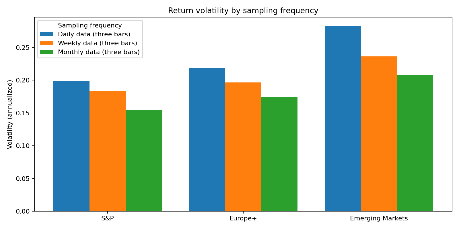
While many people are pretty aware that their horizon is monthly or even longer, people still tend to use daily data to estimate volatilities. The belief is that “more data is better, so daily volatilities are converted into monthly volatilities. The “Scaling” is done a lot in practice (even in regulatory settings).

Scaling boils down to a very simple equation: “Monthly = 21×Daily”. This works only under conditions that markets rarely meet: IID returns, constant volatility, stable correlations, and no regime changes. As we discussed before, these assumptions are highly unrealistic in practice. The chart below shows how “annualised” volatility clearly depends on the frequency of the initial data.

Estimation of Correlation:

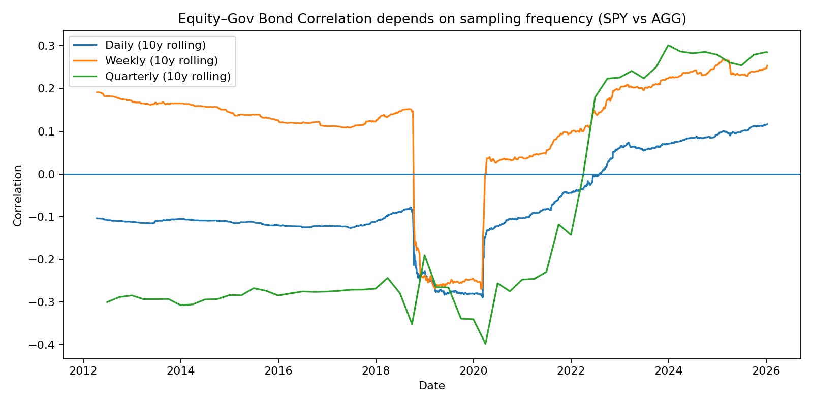
In general, please agree that correlations can strongly vary over time due to the presence of different economic regimes. However, even in the absence of regime changes, the data frequency can heavily impact the correlation estimates.

In the chart below, we present estimates of the correlation between equity and bonds based on different frequencies. Although the measures have converged in the recent period, the differences are still enough to affect portfolio allocation tremendously.

Overall, the assumption that frequency and horizon are decisions that can be made separately is incorrect. The “bridge” known as “Scaling” is more a theoretical than empirically sound approach.

Reality is the opposite: volatility clusters, correlations move with regimes, and tail dependence shows up precisely when you care about risk forecasts the most.

Even if volatility scaling is “approximately” right, dependence is not scale-invariant. Daily comovement can look very different once returns are aggregated to a monthly horizon—especially through stress periods and regime transitions.

4) Three canonical setups

To isolate the frequency/horizon effect, we keep the covariance estimator fixed (Ledoit–Wolf shrinkage) and only change how we align estimation and evaluation horizons.

A) Estimate monthly / evaluate monthly (horizon-clean)

• Estimate Σ from monthly returns (rolling 36 months)

• Evaluate risk on the 1-month horizon

• Pro: target matches the decision horizon

• Con: fewer observations → noisier estimates
  Gleichungen

B) Estimate daily / scale to monthly (common in practice)

• Estimate Σ from daily returns (rolling 756 trading days)

• Scale:

  \(Σ_{1M}≈21⋅\Sigma_{1M} \)

• Pro: more observations, typically lower turnover

• Con: dependence is not guaranteed to scale correctly
  

C) Mixed-scale (daily vol + monthly correlation)

• Estimate vol from daily data (EWMA, lambda = 0.94)

• Estimate dependence (correlation) on the monthly horizon

• Build:
  

  \(\Sigma_{1M} = Diag(\Sigma_{1D,Scaled})\,Corr_{1M}\,Diag(\Sigma_{1D,Scaled})\)

• Pro: uses daily data where it helps most (vol), keeps dependence horizon-consistent

• Con: more design choices, can increase turnover if vol is too reactive.

5) Mini case study (real ETF universe)

Universe (same as Part 1): SPY, EFA, EEM, AGG, LQD, HYG, GLD, VNQ, DBC.

Backtest: monthly rebalancing (month-end), long-only minimum-variance,

Constraints for Optimization:
(1) Max weight 60% per asset. (2) Minimum Number of Effective Assets is 3.0.

Sample: 2007-04-11 to 2026-01-09 (based on the daily close history used in the run).

Result 1: Same target horizon, different data frequency
→ different portfolio!

Do different setups produce substantially different portfolios?

Across rebalances, the portfolios from Setup A (monthly), Setup B (daily×21) and Setup C are materially different.

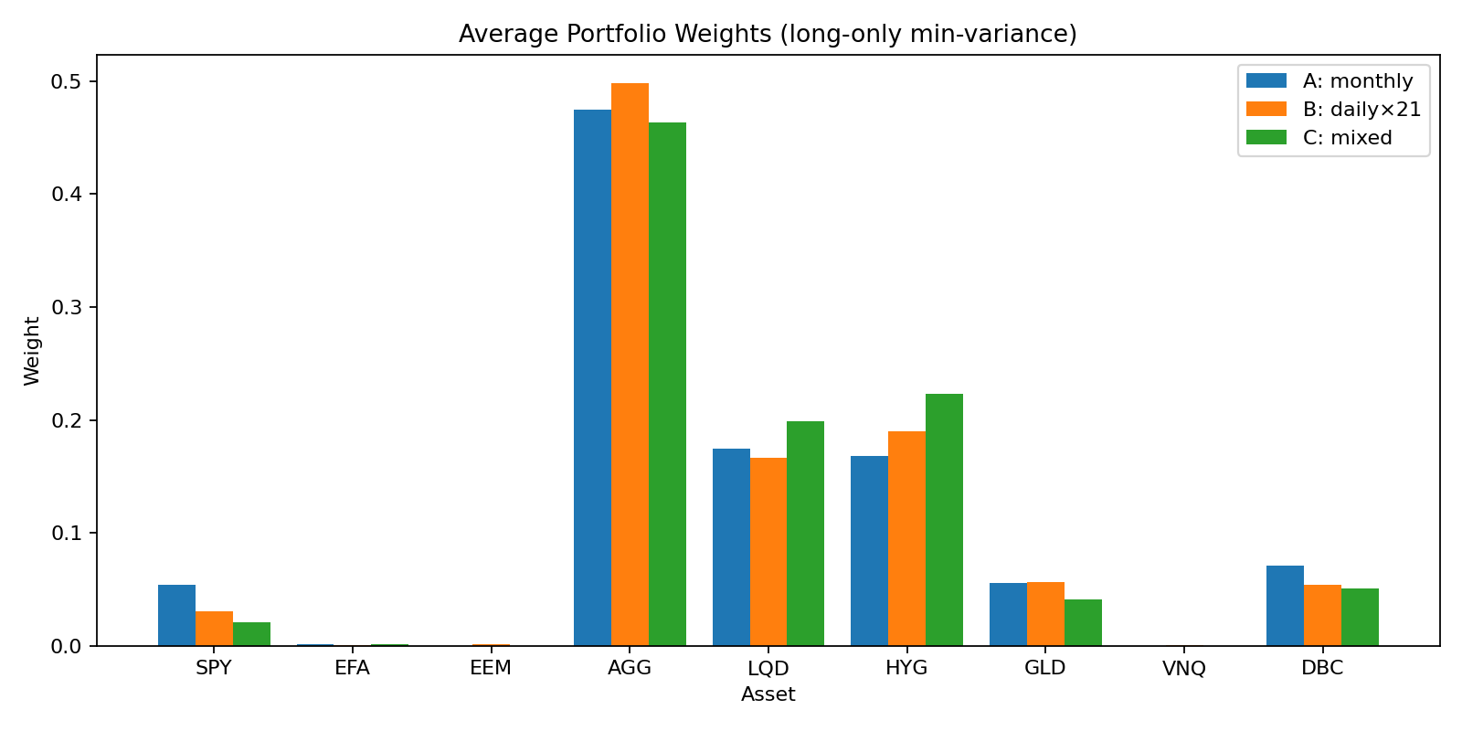
It may not “look” much but remember: (1) The scaling of the figure is in favor of underestimate the portfolio differences and (2) we have already introduced some constraints in the Minimum-Variance Optimization.

The average L1 distance between weight vectors are visualized here, when we perform rolling sample optimization.

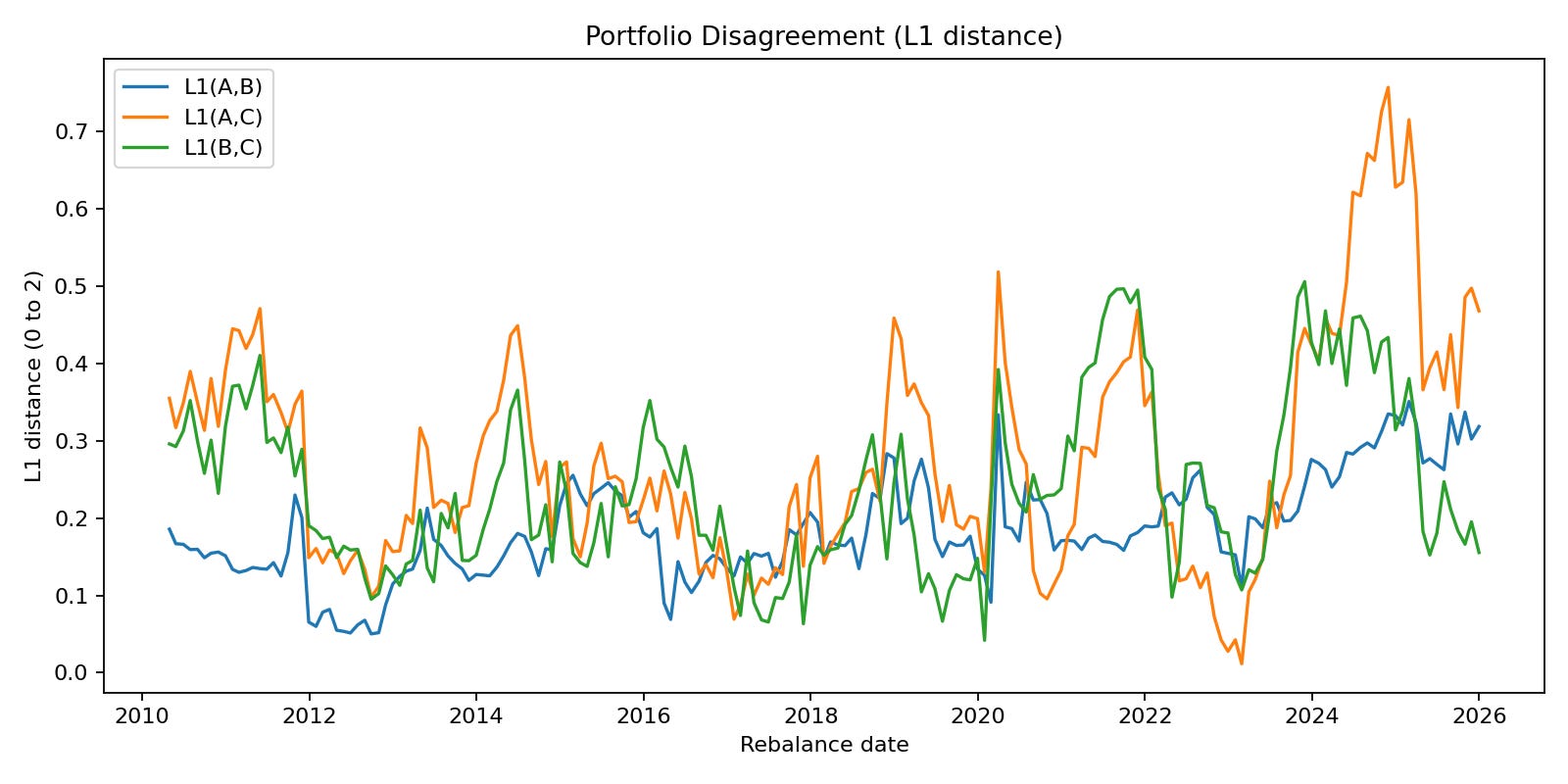
We see that especially over time, we obtain vastly “different portfolio” claim using different approaches.

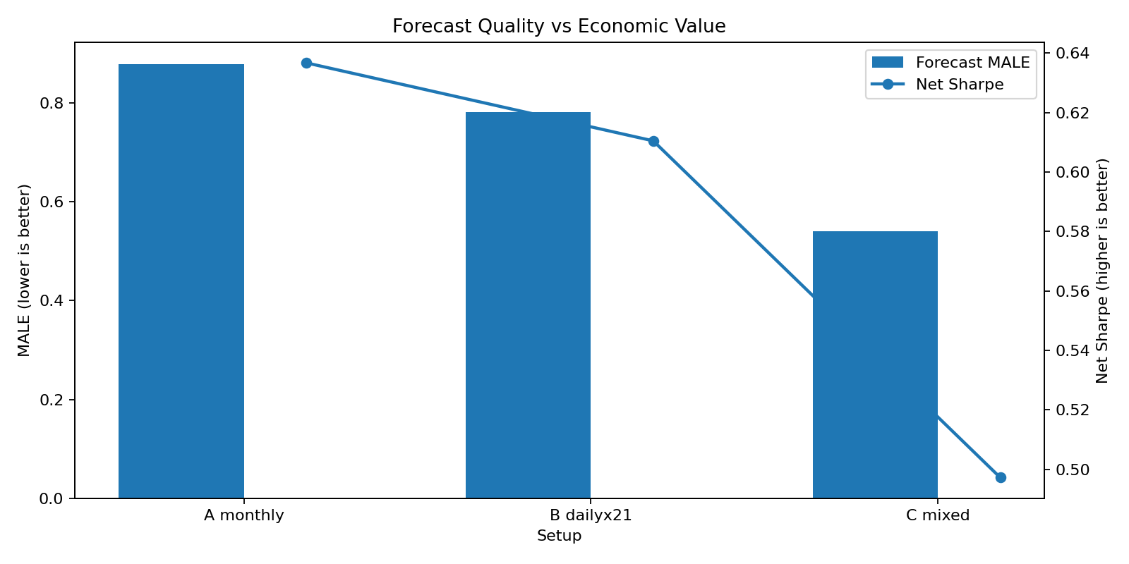
Result 2: Risk forecast quality ≠ economic quality !

Which estimator forecasts a fixed horizon better?

We estimate how well each approach forecasts the risk of its respective portfolio. We find, that the mixed approach is superior based on MALE (Mean Absolute Log Error)…but unfortunately this does not in general lead to higher economic value as measured by Sharpe Ratio. However, this result can (fortunatelly) not be generalized, but it shows that the general idea: “Better Forecasts = Better Portfolios” does not always hold.¹

We also analyse the forecast capabilities for the classic 60/40 Portfolio (Equity & Bonds) by analysing the Realized / Predicted Variance Ratio

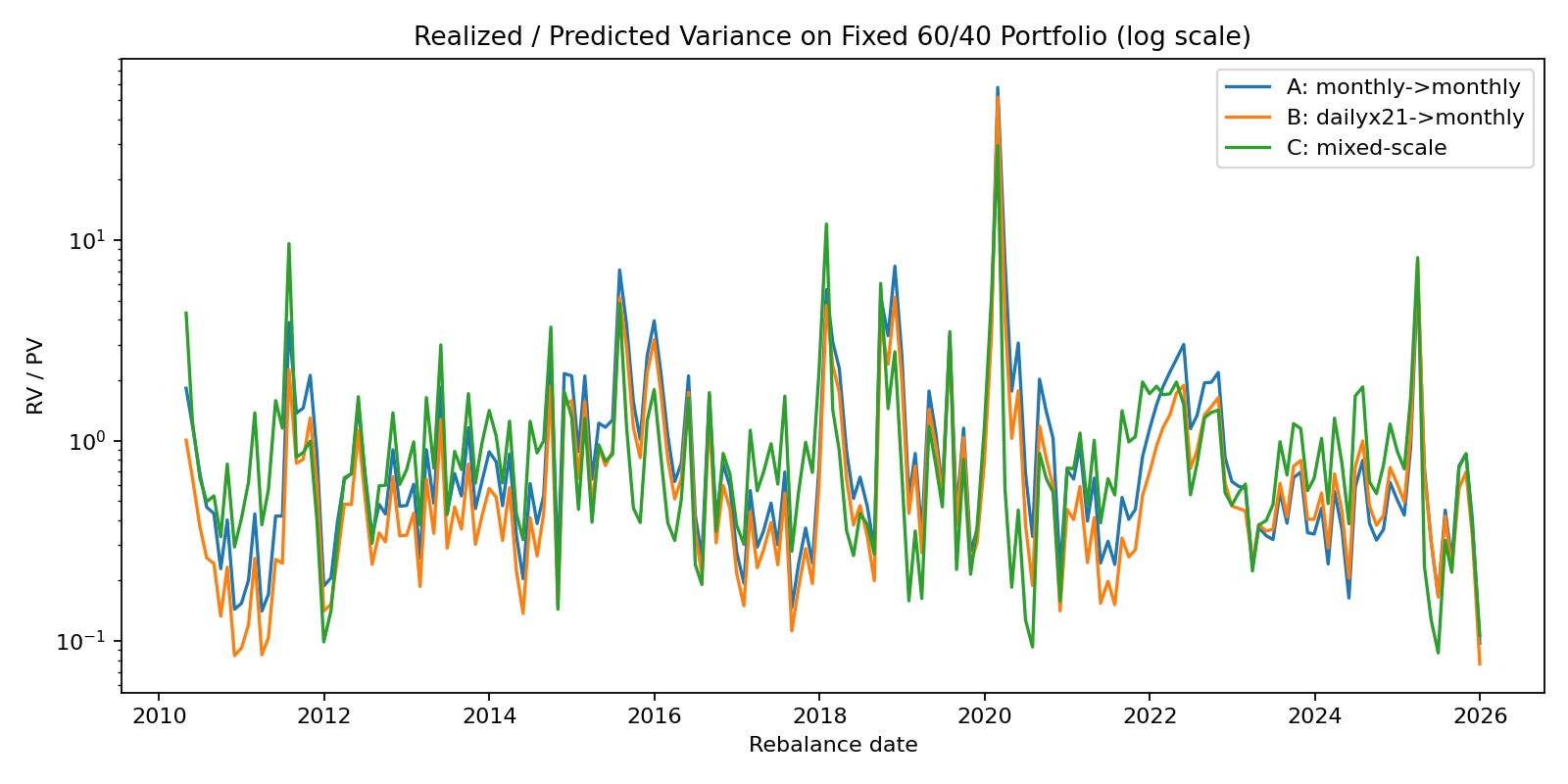
Setup B often appears more stable (lower turnover), but that does not automatically mean it is more correct for a monthly decision horizon—it can simply mean you optimized on a different dependence structure.

Result 3: …What about the Portfolio Performances?

I know what you are thinking: An analysis without a performance summary and chart is incomplete. Every Substack on Finance does this.

Let me be very clear: In many cases, presenting the performance of an estimator for a specific period (e.g. backtest) does not make sense from a statistical point of view. Judging an estimator by “which portfolio won” is the wrong approach. The experiment is about model consistency, not a horse race of realized returns. If you change the covariance estimator, you change the risk model; if you change the risk model, you change the portfolio. Period.

Those return differences are then heavily regime- and path-dependent noise around the actual point: whether your estimator reflects the horizon you are investing on. Treating a short sample performance spread as proof that one estimator is “better” is category error. The real failure is horizon mismatch, because that is what systematically drives mismeasured risk and unstable allocations.

6) Practical rules of thumb

1. Decide the horizon first (rebalance schedule defines your risk target).

2. Evaluate on that horizon (otherwise you can’t compare models fairly).

3. Treat scaling (“×21”) as a model assumption, not a law of nature.

4. If you must use daily data, use it primarily for volatility, not blindly for dependence.

5. Mixed-scale models are often a good compromise: daily vol + horizon-matched correlation.

6. Watch out for “improvements” that are really just frequency artifacts (lower turnover is not proof of better horizon risk).

7. Write down the horizon contract: “This Σ forecasts 1-month risk under monthly rebalancing.”

7) Summary & Teaser to the next Article

• Horizon ≠ frequency.
  Data frequency is a measurement choice; horizon is the portfolio’s objective.
  Do you want your portfolio to be diversified for the long-run or short-run? Is both possible?² Estimator choice is a horizon choice; frequency-mismatched covariance produces different portfolios, even with the same optimizer
  

• Scaling is fragile
  Autocorrelation, volatility clustering etc. violate the IID assumption of asset returns. This makes scaling from one frequency to another by using the “scaling equation” very fragile. In addition: Dependence structures (e.g. correlations) are also are not scale invariant in real markets and very with data frequency.
  

• Fix the horizon first—then evaluate estimators in portfolio space.
  Focus on the things that are given first. If a portfolio has a long-term objective, this factor should then be a cornerstone of you approach to estimate parameters and optimize the corresponding portfolio.

Part 3 of the Covariance Series: Now that the horizon is well-defined, we can finally compare estimators where it matters: risk forecast error, turnover, and concentration. Evaluation of estimators inf portfolios space will be part of the next article.

1. It is important to note that looking better in one specific metric does often not tell the entire story.

2. Spoiler: Yes, it is to a certain degree.